SOLVING OPTIMIZATION USING GENETIC ALGORITHM

INTRODUCTION

WHAT IS AN OPTIMIZATION PROBLEM?

Optimization problems are the ones in which we need to find the maxima or minima of a function. Example iterating the value of Engine-Piston parameters for better efficiency. In this report, we are focusing on one of the evolutionary algorithms which are used to solve these kinds of problems called the genetic algorithm, and how varying its parameters change the computational time and efficiency of the solver.

WHAT IS THE GENETIC ALGORITHM?

The Genetic Algorithm (GA) is a part of a broader classification of algorithms called the Evolutionary algorithm which mimics the evolution of the life process, proposed by Charles Darwin, to find a solution for a problem without dwelling on its derivative information.

It follows the below steps:

1. Generating initial population
2. Evaluating the fitness of the individual(chromosomes)
3. Selection of the fittest
4. Crossover
5. Mutation
6. Termination

GENERATING INITIAL POPULATION

The initial population is generated by randomly mixing various combinations of the inputs. The more the population generated, the more the accuracy but also more the computational time.

EVALUATING THE FITNESS OF THE INDIVIDUAL

After the population is generated, each individual is evaluated based on the fitness function (Function which provides criteria). After the evaluations, scores will be generated which gives their probability to proceed further.

SELECTION OF THE FITTEST

Based on the fitness score, two pairs of individuals will be selected for the crossover.

There are different types of selection. Some of them are explained below.

1. Random Selection- each individual in a particular set is selected randomly.
2. Tournament Selection- In this several tournaments will be conducted on the population set and k number of the best individuals will be selected like this several tournaments will be conducted and the best of all the tournaments will be selected as parents. In this method, the individuals having weaker scores are eliminated.
3. Roulette wheel Selection- In roulette wheel selection each individual will have a probability based on their fitness function and like a roulette game, individuals will be selected randomly. If the probability is more, then the chance of selection is also more.

CROSSOVER

In this step, the parameter of the individuals (Genes) will be shuffled based on a randomly generated point called the crossover point. The resulting two individuals will be called off-springs.

There are different types of crossover. Some of them are given below.

1. Single-point crossover- In this, the chromosome sets are split into two sections and one of the sections from each set interchange their sections correspondingly.
2. Two-point crossover- Here, the chromosome sets are split into three sections, and one of their three sections gets interchanged.
3. Multi-point crossover- This is a general case of two-point crossover where the chromosome sets are split into n+1 sections and n-1 sections will be interchanged correspondingly
4. Uniform Crossover- In this, each bit in chromosome sets is selected randomly and interchanged with its corresponding bits.

MUTATION

In this step, some of the genes will be changed randomly to maintain diversity in the population and prevent premature convergence.

TERMINATION

This process will be repeated again and again until it reaches the termination condition where the population converges. This is to prevent a significant difference in population which can cause an overshoot causing erroneous results and long computational time.

STRUCTURE OF GA

fun- The function for which we need to find the minimum. It is also the fitness function.

nvars- It specifies the number of variables that the function has.

A and b – Linear inequality constraints, these are matrix form of sets of equations where A is the coefficients of the variables and b is the right-hand side values of the inequality operator.

A_eq, b_eq- Same as A and b but instead of inequality constraints it works under equality constrains.

lb, ub- Lower and upper bounds for the variable. It helps us to reduce the search area and increase the result consistency.

nonlcon- These are used to provide the non-linear constraints for the variables. (c, c_eq)- c is for non-linear inequality and c_eq is for non-linear equality.

Options- This contains what are the parameters that we have set for ga. One of the options which is used in this code is given below.

PopulationSize- This helps to control the population count at each iteration.

CODE EXPLANATION

The purpose of the code is the find the global maxima of the stalagmite function and to explore how adding the constraints to GA helps in getting better results.

The code is split into three parts

• Global_Maxima_Optimization_Code.m – master code
• stalagmite.m and - subFunction
• GA_statistics.m – subfunction

Stalagmite

function [result] = stalagmite(a)
%This is the function for which maxima value has to be found.This is the function for which maxima value has to be found.
%a input vector[a(1)-x,a(2)-y]
f_1x=(sin(5.1*pi*a(1)+0.5))^6;
f_1y=(sin(5.1*pi*a(2)+0.5))^6;
f_2x=exp(-4*log(2)*(a(1)-0.0667)^2/0.64);
f_2y=exp(-4*log(2)*(a(2)-0.0667)^2/0.64);
result=-(f_1x*f_1y*f_2x*f_2y);
end

This is the function for which maxima value has to be found. The mathematical form of the function is given below.

`f_1x=(sin(5.1*pi*a(1)+0.5))^6`

`f_1y=(sin(5.1*pi*a(2)+0.5))^6`

`f_2x=exp(-4*log(2)*(a(1)-0.0667)^2/0.64)`

`f_2y=exp(-4*log(2)*(a(2)-0.0667)^2/0.64)`

(GA can find only the global minima of a function hence a negative sign is used in the result to convert the global maxima to global minima. By this way, we can find the global minima of the function)

Here a(1) and a(2) represents the variable x and y.

The input for this function will be the x and y variables which will be fed by the GA algorithm.

GA_statistics

function [] = GA_statistics(x_v,y_v,fval,k,title_text)
%This function is to plot the graph that are required for better representation of the result.
%% Code Parameters
% xx,yy-2-D mesh grid
% input_vector- input parameter for stalagmite function.
% f-Stalagmite Result
% x_v-x value of maxima
% y_v-y value of maxima
% fval- maxima value
% tittle_text- title for the graph

x_low=0;
y_low=0;
x_max=0.6;
y_max=0.6;
sampleSize=150;
x=linspace(x_low,x_max,sampleSize);
y=linspace(y_low,y_max,sampleSize);
%% Stalagmite Values

[xx, yy]=meshgrid(x,y);
for i=1:length(xx)
    for j=1:length(yy)
        input_vector=[xx(i,j),yy(i,j)];
        f(i,j)=stalagmite(input_vector);  
    end
end
%% GA_Plot

figure(k)
sgtitle(title_text)
subplot(2,1,1)
hold on
surfc(xx,yy,-f)
shading interp
plot3(x_v,y_v,-fval,'marker','o','markersize',5)
subtitle("Stalagmite Surface with Maxima Value on each Iterations")
hold off
subplot(2,1,2)
plot(-fval)
axis([0 150 0 1])
xlabel("Number of Iterations");
ylabel("Maxima Value");
subtitle("Number of Iterations vs Maxima Value");
end

This function is to plot the graph that is required for a better representation of the result. This function is divided into three sections.

• Code Parameters
• Stalagmite Values
• GA_Plot

Inputs for the function

x_v-x value of the global maxima.

y_v- y value of the global maxima.

fval – Maxima value

k- Figure Number

title_text- Title of the graph

Code Parameters

This section is to provide the range and sample size of the variables x and y required to plot the stalagmite function.

Stalagmite Values

This section converts the x and y variables into two dimensional mesh grid which is then provided as input parameters for the stalagmite function. It generates the values for stalagmite function.

{code}

GA_Plot

This section contains code for surface plot of stalagmite function and also contains a general format for plotting graph for all three studies.

It contains the plot for x_v, y_v and feval which overlaps on the surface function for better understanding of the GA’s behaviour.

{code}

Global_Maxima_Optimization_Code

clear all %#ok<CLALL> 
close all
clc

%% Input
% Terminology
% LowerBound of data x and y "l"
% UpperBound of data x and y "u"
% X-value of the data x_v
% Y-value of the data y_v
% stalagmite-Function
% start of timer for studies - study_{study number}_time_start
% end of timer for studies - study_{study number}_time_end
% maxi-location of maxima value(x,y)
% fval-maxima value
% GA_statistics-For ploting the graph
num_cases=150;
nVar=2;
l=[0;0];
u=[0.6;0.6];
%% Study-1:No Constraints
study_1_time_start=tic;
for num_iter=1:num_cases
[maxi,fval(num_iter)]=ga(@stalagmite, nVar); 
x_v(num_iter)=maxi(1);
y_v(num_iter)=maxi(2);
end
GA_statistics(x_v,y_v,fval,1,"No Constraints");
study_1_time_End=toc(study_1_time_start);
clear('x_v','y_v','fval','maxi');
%% Study-2:With lower bounds and upper bounds
study_2_time_start=tic;
for num_iter=1:num_cases
[maxi,fval(num_iter)]=ga(@stalagmite, nVar,[],[],[],[],l,u);
x_v(num_iter)=maxi(1);
y_v(num_iter)=maxi(2);
end
GA_statistics(x_v,y_v,fval,2,"With lower bounds and upper bounds");
study_2_time_End=toc(study_2_time_start);
clear('x_v','y_v','fval','maxi');
%% Study-3:With lower bounds, upper bounds and populationSize
options=optimoptions('ga');
options=optimoptions(options,'PopulationSize',300);
study_3_time_start=tic;
for num_iter=1:num_cases
[maxi,fval(num_iter)]=ga(@stalagmite, nVar,[],[],[],[],l,u,[],[],options); %#ok<*SAGROW> 
x_v(num_iter)=maxi(1);
y_v(num_iter)=maxi(2);
end
GA_statistics(x_v,y_v,fval,3,"With lower bounds, upper bounds and populationSize");
study_3_time_End=toc(study_3_time_start);
clear('x_v','y_v','fval');
%% Display Time
disp(study_1_time_End);
disp(study_2_time_End);
disp(study_3_time_End);

figure(4)
bar([study_1_time_End,study_2_time_End,study_3_time_End])
title("Time statistics")
xlabel("Study")
ylabel("Time taken")

This code is divided into four sections

1. Input
2. Study-1:No Constraints
3. Study-2:With lower bounds and upper bounds
4. Study-3:With lower bounds, upper bounds and populationSize
5. Display Time

Input

This section explains the variable name and sets values to the parameters required for GA.

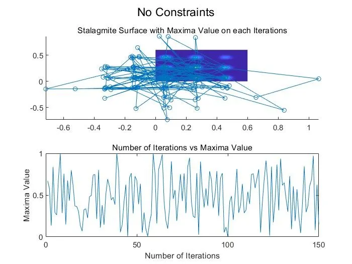
Study-1:No Constraints

In this section, there are no constraints given to the GA other than the stalagmite function as with function handler and the number of variables. As we can see from the plot the feval values are spread all over the places in the plot each time the GA runs.

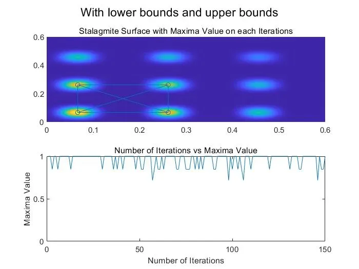
Study-2:With lower bounds and upper bounds

In addition to the parameters given in study-1, the upper and lower bounds for the variables are added to the GA. This greatly improves the consistency of the results but still the results are oscillating between some few values.

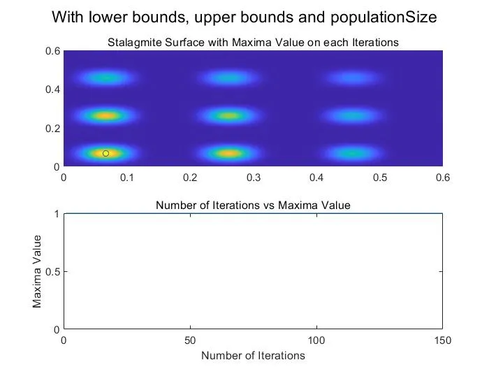
Study-3:With lower bounds, upper bounds and populationSize

The options parameter is added to the GA from study-2. The options parameter is given value by the “optimoptions” code. The optimoption first takes the parameter GA to indicate that we feed the options of GA. In the next line using the same code options is passed again with populationSize as a parameter. This further enhances the reliability of the code and provides the consistent result.

Display Time

For each section the computation time taken is calculated and it is displayed in the command line prompt and as a bar chart.

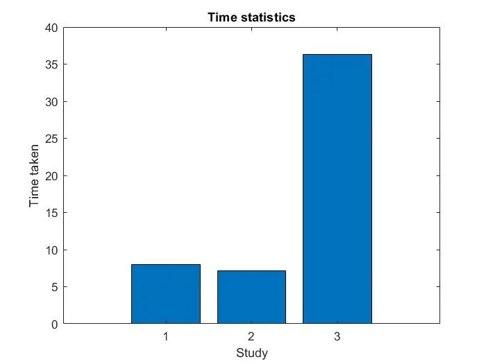
As you can see from the graph tough adding constraints increases the reliability it also needs more computational power and requires more computational time

ERROR OCCURRED DURING THE CODE

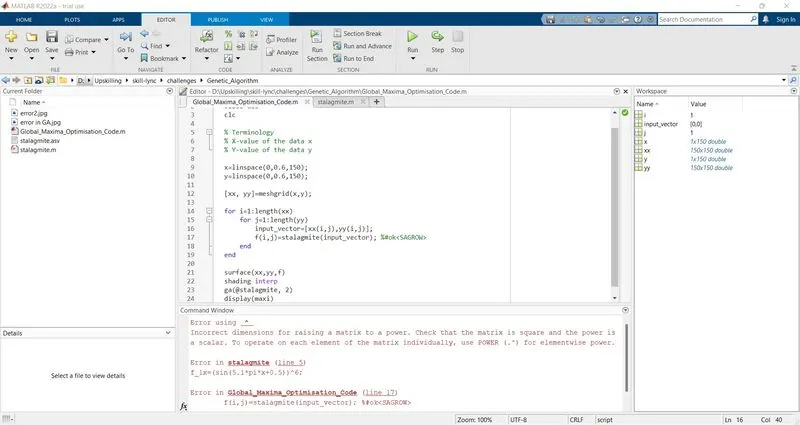
Used given two variables as separate 1x1 matrices instead of one 2x1 matrix containing both x and y variables.