Week 3 - Solving second order ODEs

% problem to solve second order ODE for pendulum in MATLAB.

# introduction: Simpal pendulum is as shown in figure,

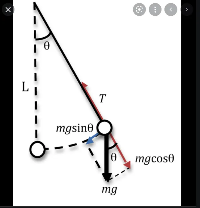
here,

L= length of string

theta=displacement

mg= W= weight of pendulum

pendulum is a weight suspended from a pivot so that it can swing freely.When pendulum is displaced isideway from its resting ,equilibrium position ,it is subjected to arestoring force due to gravity that will accelerate it back towards the equilibrium position.

# Ordinary Differencial Equation

- In science and engineering ,most of the phenomenon and fundamental laws are explained with the help of differencial equations .

-Differencial equations describes the changes in the state of system.They express the relation between vaariable based on diffencial calculas.

-When diffrencial equations contains all the derivatives with respect to singal varialbles,then it is called as an 'Ordinary Differencial Equations'.

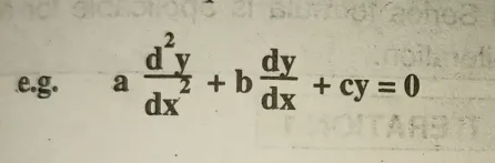
-The above equation contains derivative with respect to x only,hensce it is called as an ordinary differencial equation.

# the ODE used for pendulum is

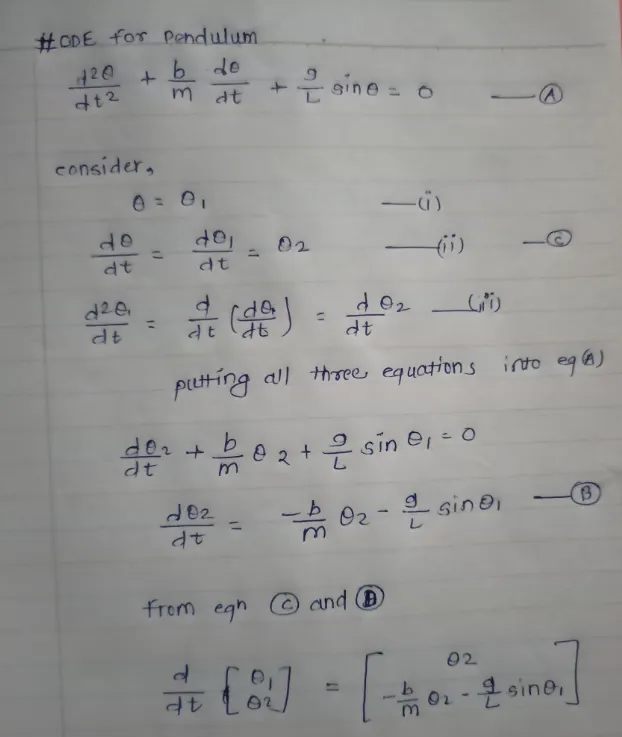
here ,we have to convert the second order differencial equations into the first order.

# code for ode

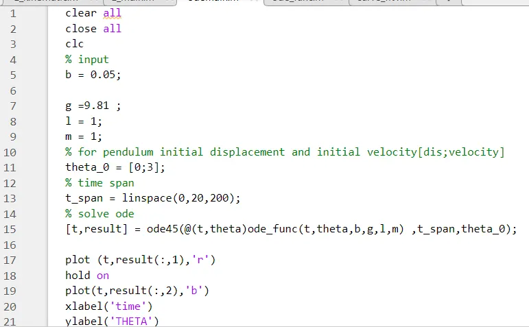
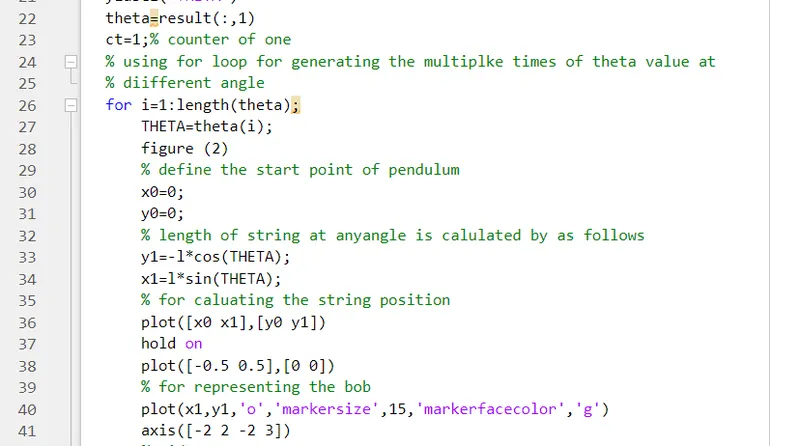
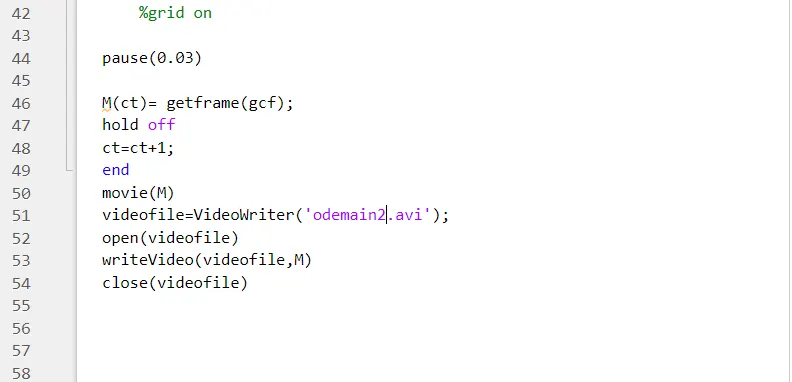
#code function

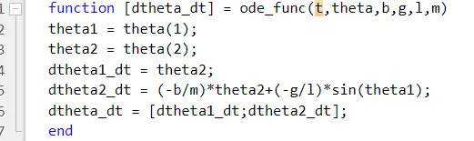
# code explanation

always start with clear all,close all ,clc

after that define the damping coefficent (b),length of rod(l) in meter ,mass of pendulum(m) in kg

Then give the initial values for displacement and velocity i. e theta=[0;3]

With help of linspace command generate the array for 't'

ODE45 function= ODE45 is usually the function of choice among the ODE solvers.It compares methods of orders four and five to estimate error and determine step size.for simpal,ode45 solves the system to produce results for each initial value.

use ode45 to create the the function and then use it in main program

here ode45@(t,theta )means it is the function of time and displacement(theta)

ode_func(input_vector ) is the function generated in matlab

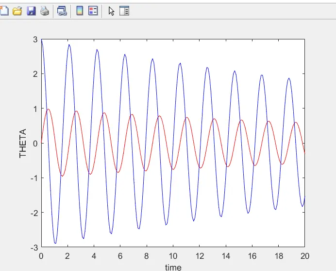
affter that we have to plot figure 1 Displacement and velocity with respect to time.for that select the all rows and one by one two columns for two different plot commands .Then give the legends and title and labels to axis

for making the animation on matlab we have to use' for loop' for generating the sereis of plots for length of theta

In next step define the points at hinge that is initial condition.Also define the linear displacement of bob by using the trigonametric equations.

Then use pause command to pause the every loop after each value.then use counter =1 for increment in each event ,then end the for loop.

Use movie command as per code to create a video. that file must be stoared in project.avi format

#errors

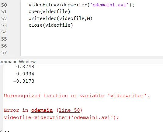
BOTH the errors i faced because of wrong spelling

error 1-this error i got because of the videofile pelling in line 49

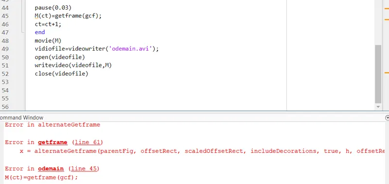
Error 2=

in videowriter command always make sure that 'V'and 'W' must be capital.

-

both the errors are solved by support engineer at skill lynk.

# output plot

From the graph we clearly known that as the damping coefficient increases the damping effect also increases means we get less oscillation

# link for animation

https://drive.google.com/file/d/1ky8En6g0jMcdvql-AM-32NpJoq0UyO7i/view?usp=sharing