Week 3: Flow over a backward facing step
AIM:- SIMULATE THE FLOW OVER BACKWARD FACING :-
OBJECTIVE:-
. Run 3 simulation
. with 3 different base mesh sizes are
1. dx = 2e-3m dy = 2e-3m dz = 2e-3m
2. dx = 1.5e-3m dy = 1.5e-3m dz = 1.5e-3m
3. dx = 1.0e-3m dy = 1.0e-3m dz = 1.0e-3m
Contents to shown in the report:-
1. Show the mesh for all the 3 base mesh sizes
2. Show pressure and velocity contours
3. Show the plots of velocity ,pressure,mass flow rate,and totall cell counts for all the 3 base mesh sizes
4. Also explain where and why separation is talking place in detail
INTRODUCTION:-
The backward-facing step is widely used for its application of turbulences in internal flows.the flow separation is casued due to the sudden changes in the geometry and the inlet and outlet pressure values the flow separation causes a point of reattachment and a point of recirculation
The backward - facing step represents separation flows which can be widely seen in aerodynamic flows heat transfer,engine flow, condensers vehicles and flow around the building.
Geometry:-
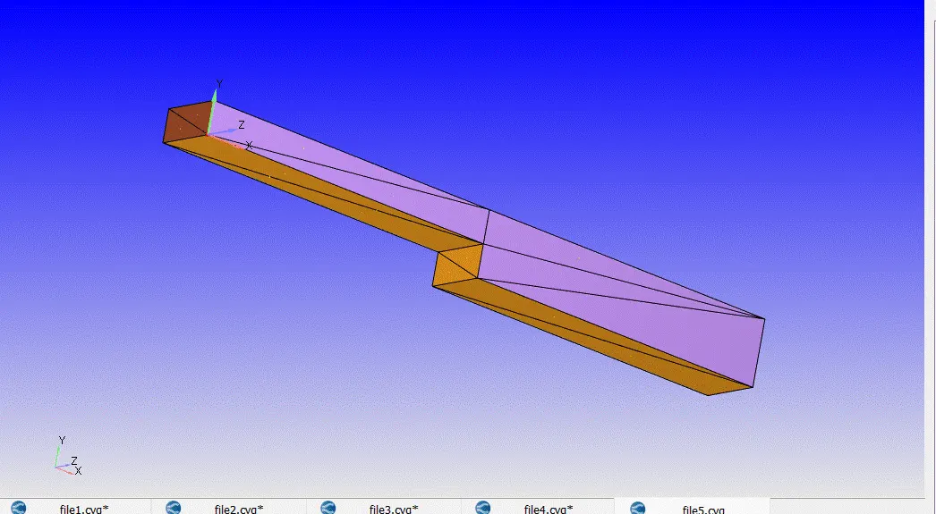
1. created geometry of backward facing step
2. Checking the normal
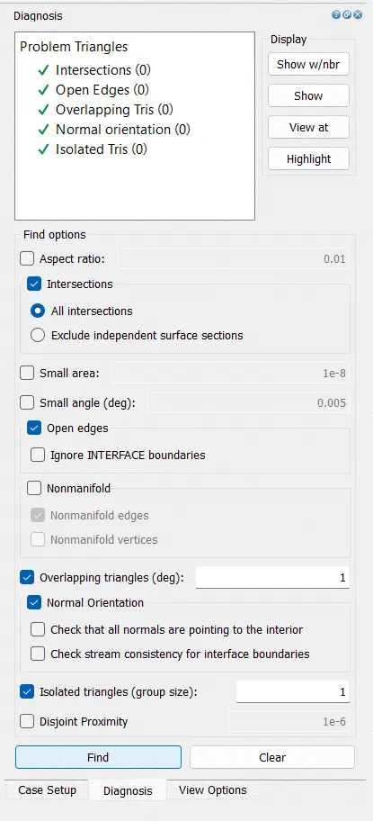
3. Checking the diagnosis in order to checks error
Before proceeding the error in geometry for that
View tab-diagnosis dock-default setting-select the find
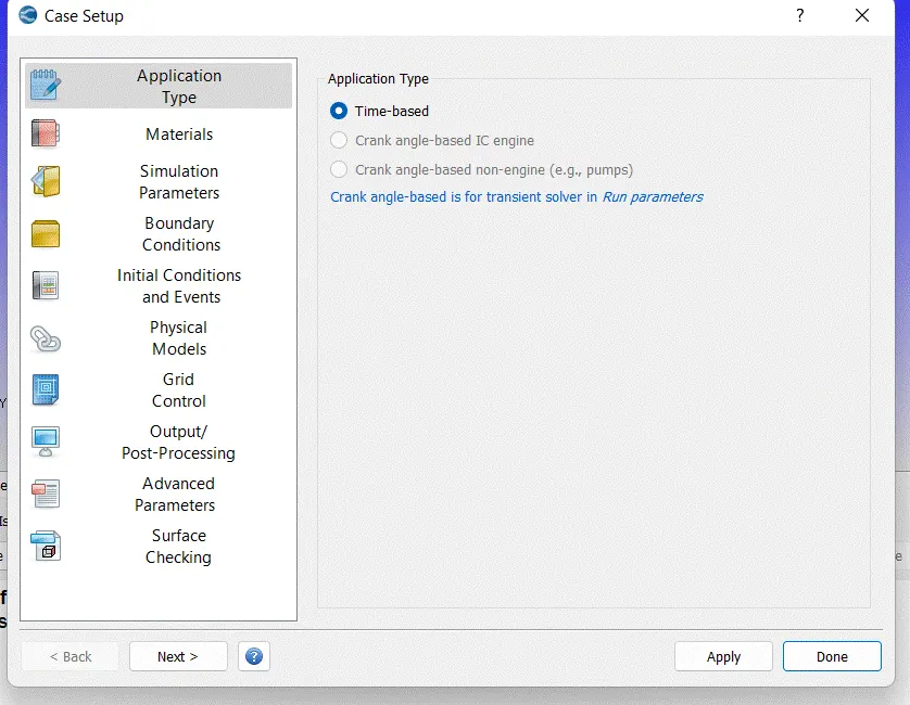
Case setup:-
Application Type:- Time-Based
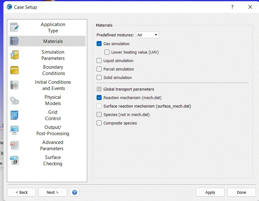
Marerial :-
Predefind mixture:- AIR
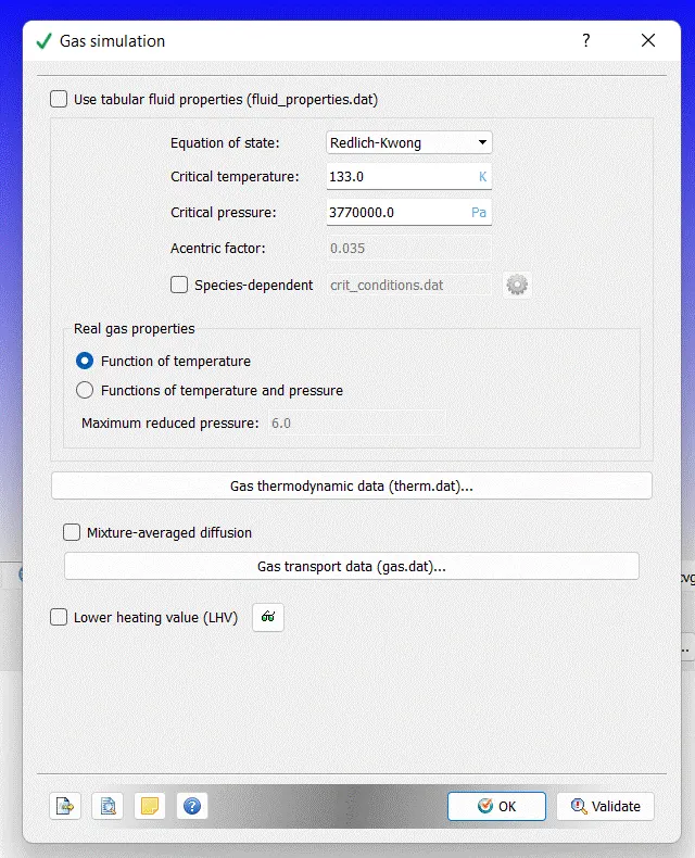
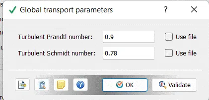
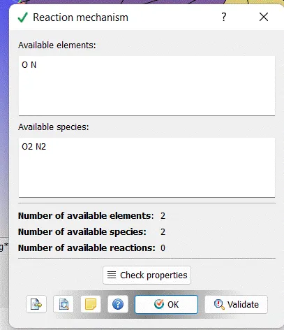
Simulation Parameters:-
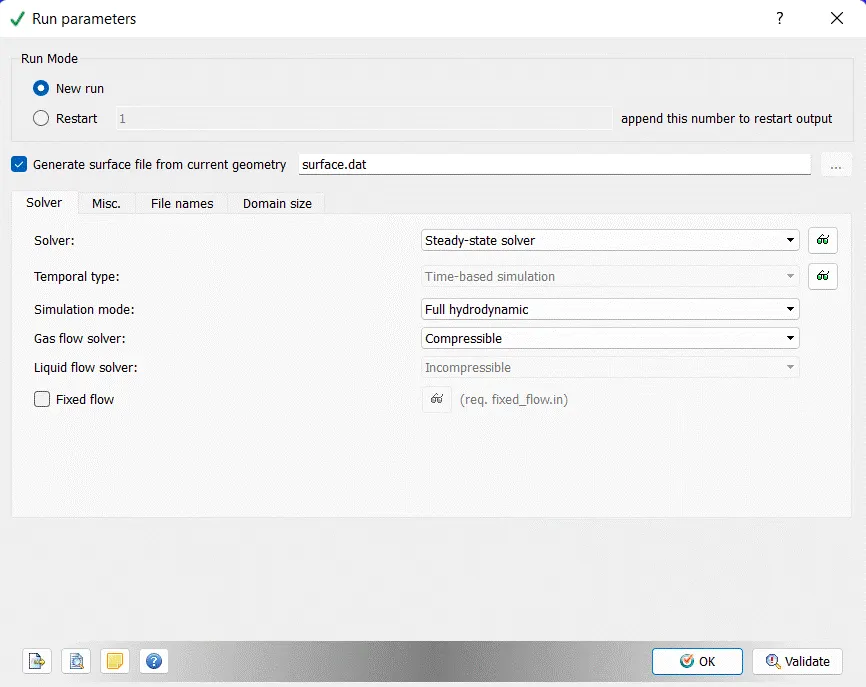
In Run Parameters Two Main Things To Be Considered
Select the following solver settings.
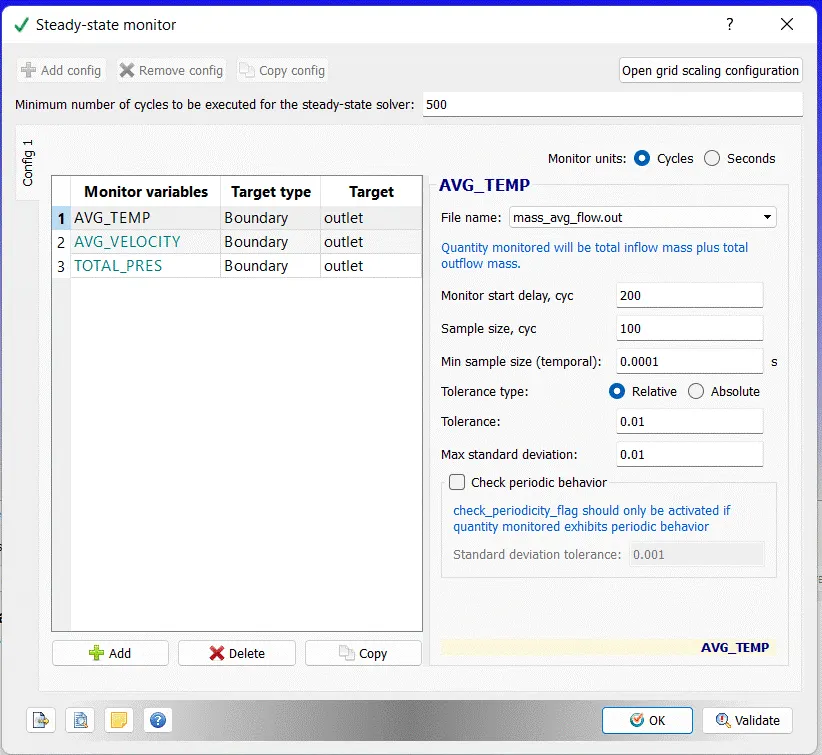
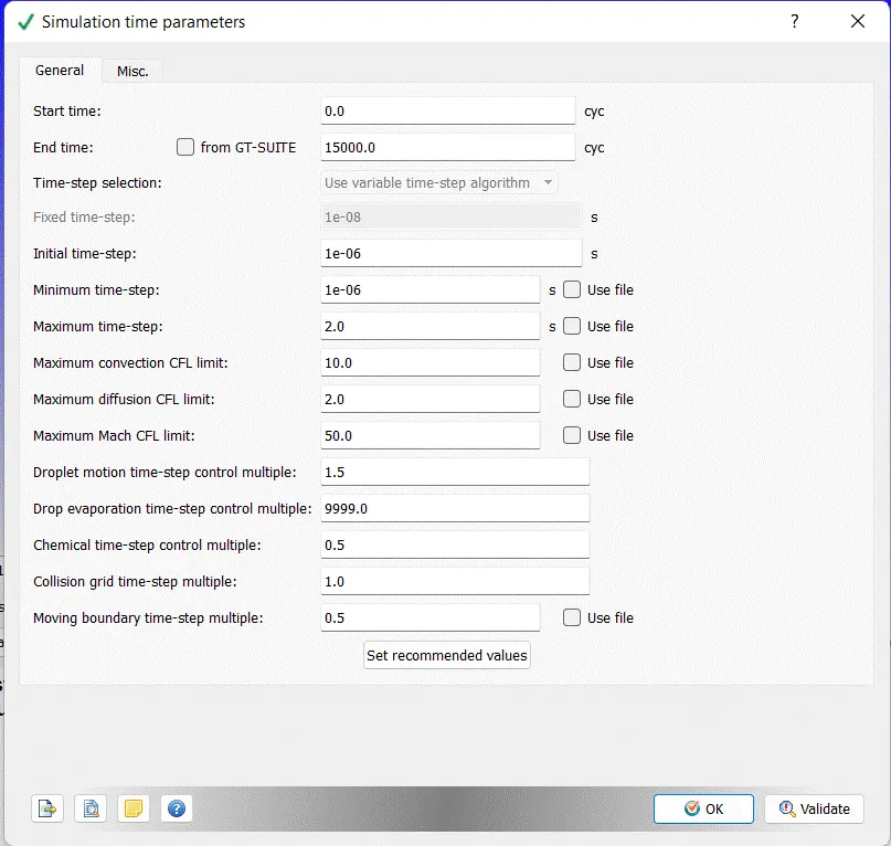
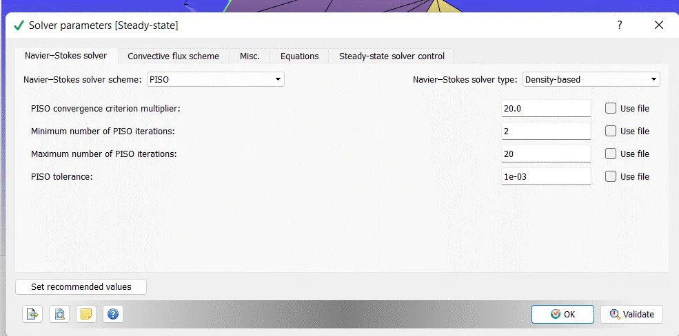
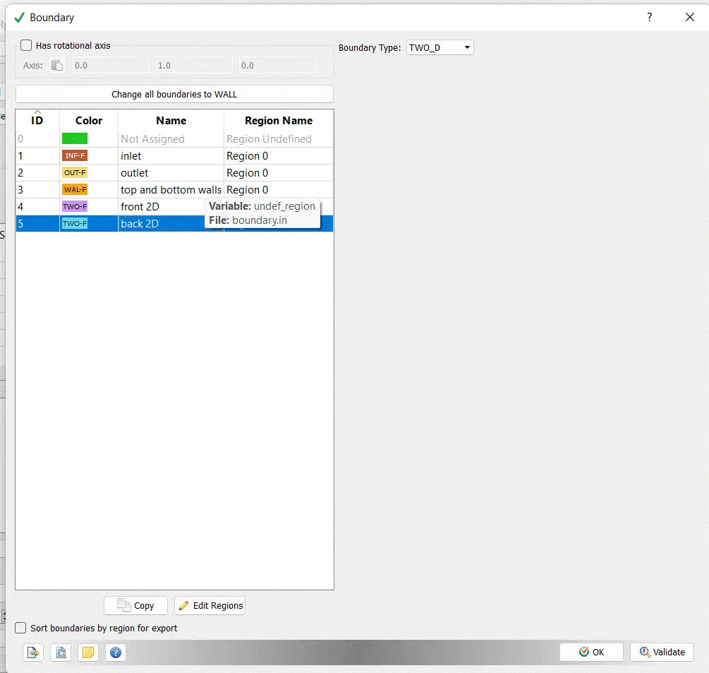
Click on the Boundary to Creat Boundarys:-
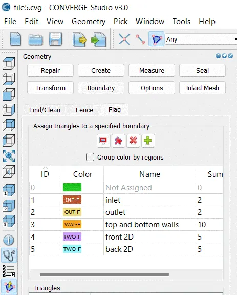
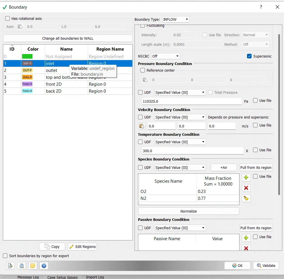
Inlet :-
Boundary type:- INFLOW
Region name :- Region 0
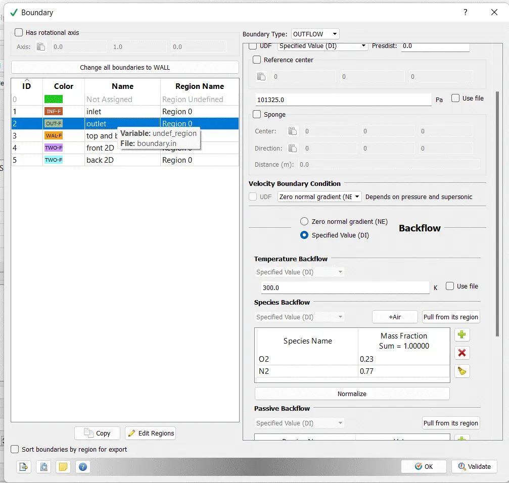
Outlet:-
Boundary Type :- OUTFLOW
Region name :- Region 0
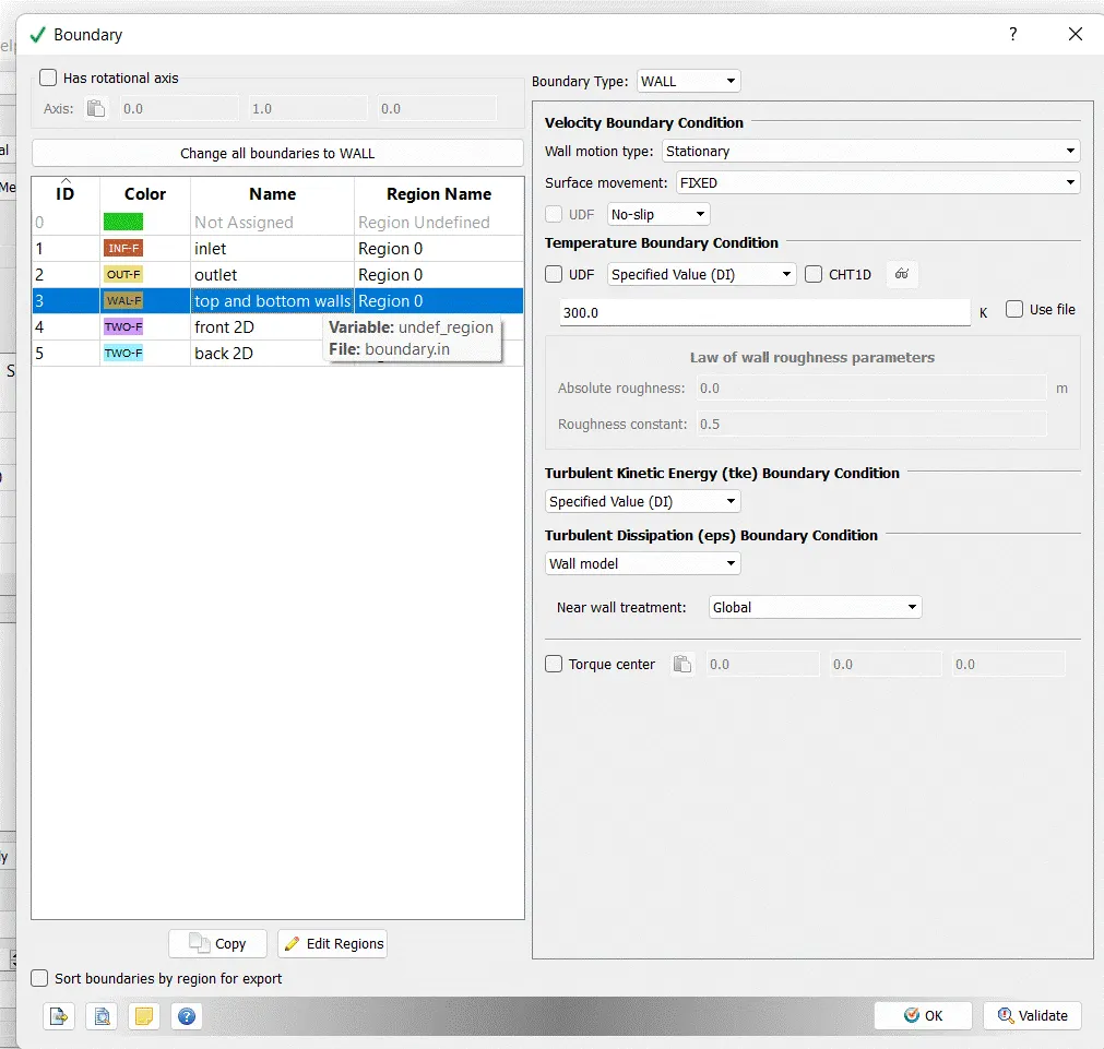
Top and Bottom Walls :-
Boundary Type :- WALL
Region name :- Region 0
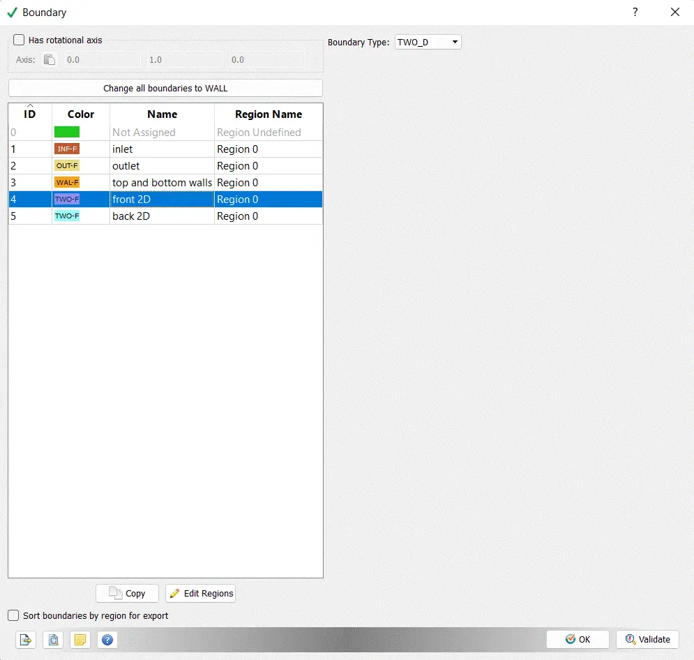
Front 2D :-
Boundary Type :- TWO_D
Region name :- Region 0
BACK 2D :-
Boundary Type :- TWO_D
Region name :- Region 0
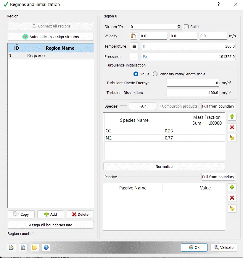
Region and initialization:-
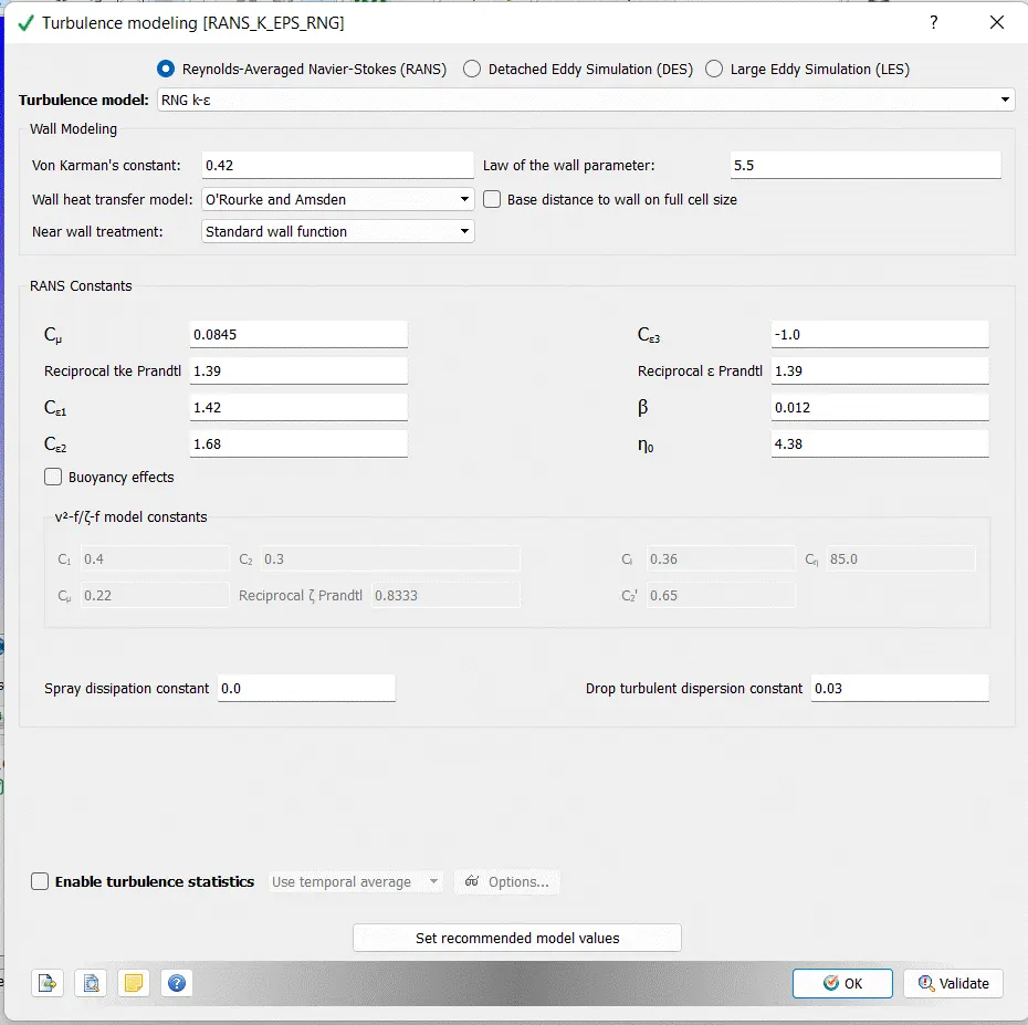
Turbulence Modeling:-
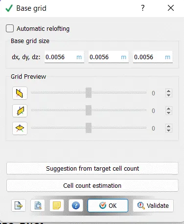
Base Grid:-
Case:- dx = 2e-3m dy = 2e-3m dz = 2e-3m
Case:- dx = 1.5e-3m dy = 1.5e-3m dz = 1.5e-3m
Case:- dx = 1.0e-3m dy = 1.0e-3m dz = 1.0e-3m
NOTE:- change base grid size according to your setup
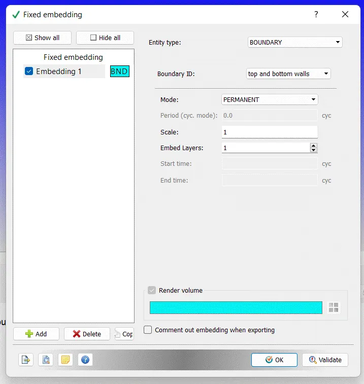
Fixed Embedding :-
Entity Type:- BOUNDARY
Boundary ID:- TOP AND BOTTOM WALLS
Mode :- PERMANEENT
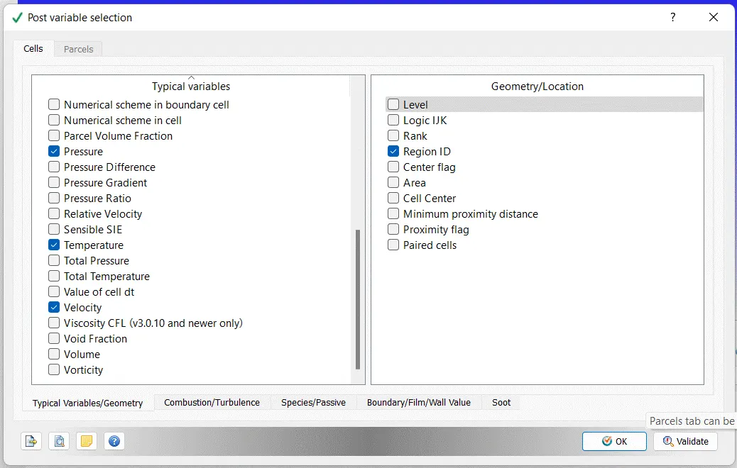
Post Variable Selection:-
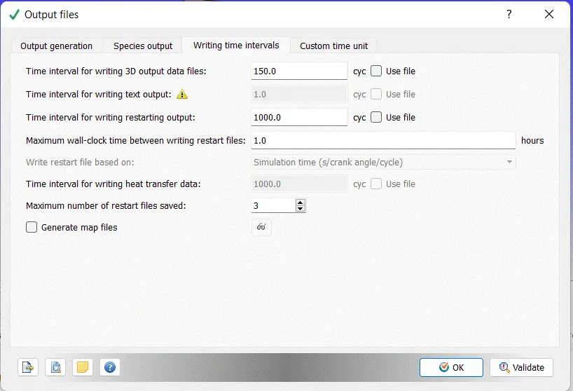
OutPut Files:-
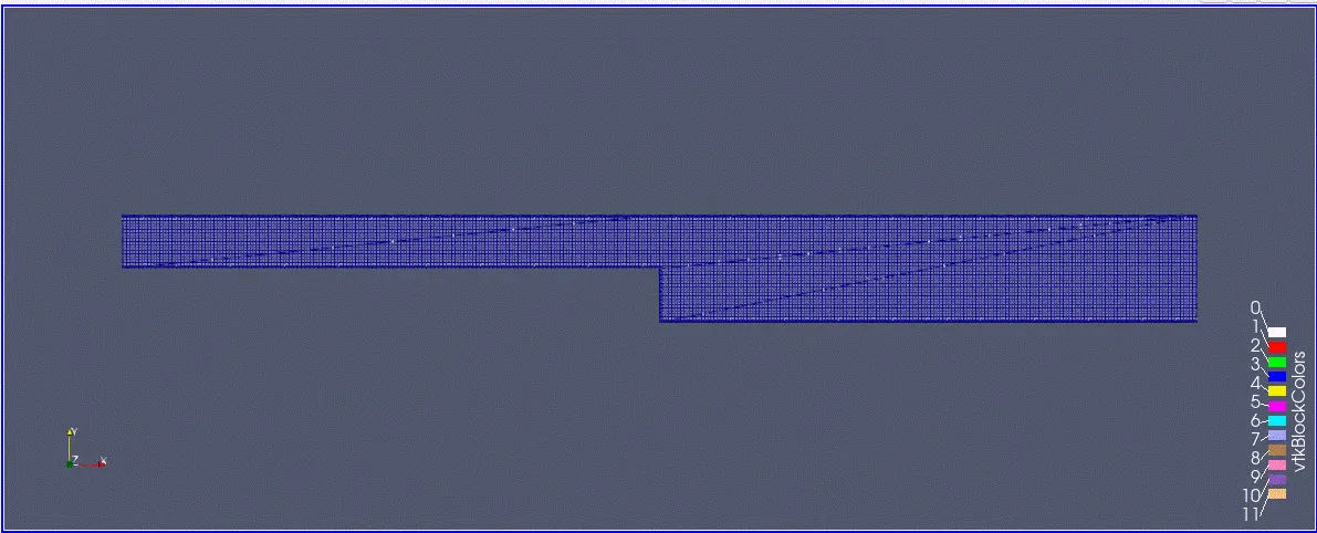
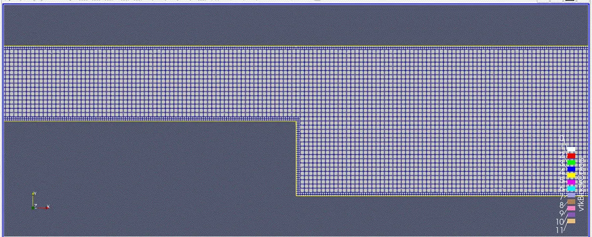
Mesh:-
Case:- dx = 2e-3m dy = 2e-3m dz = 2e-3m
NOTE:- change base grid size according to your setup
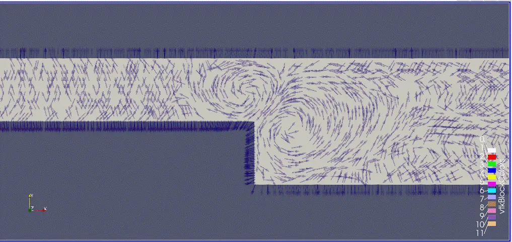
Velocity Vector near Recirulation:-
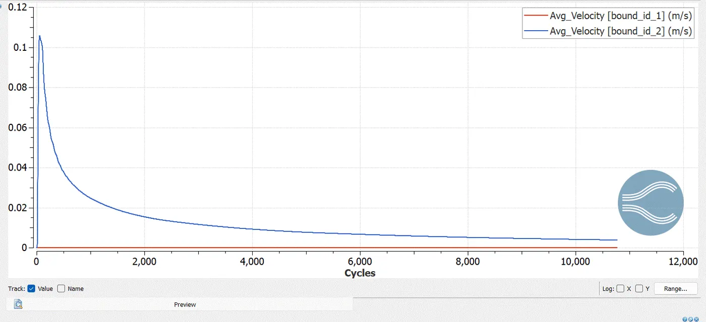
Velocity plot:-
Input and Output
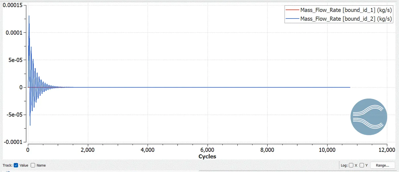
Mass_Flow_Rate Plot:-
Input and Output
Pressures Plot:-
Inlet and Outlet
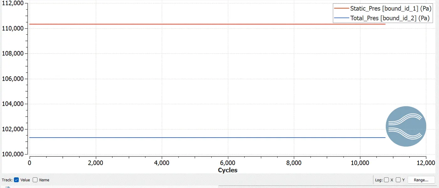
Velocity Plot:-
Inlet and Outlet
Total cells Counts :-
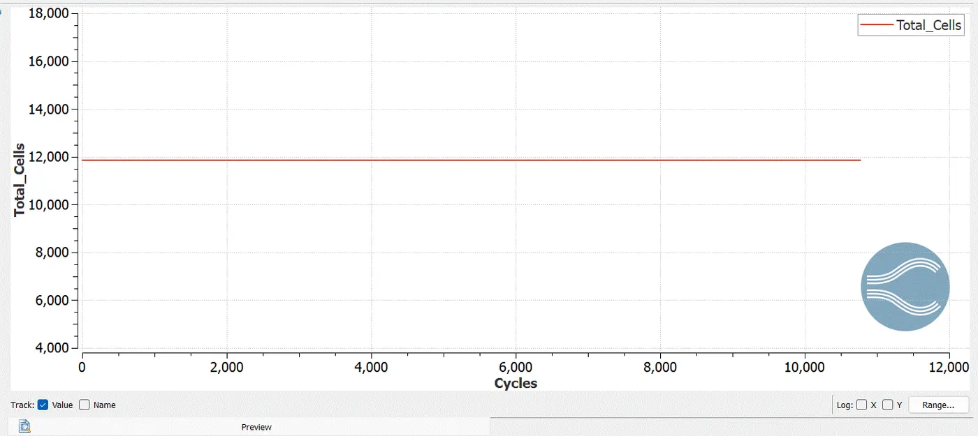
Velocity Contour:-
Pressure Contour:-
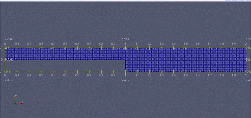
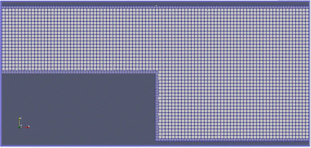
Mesh Grid:-
Case:- dx = 2e-3m dy = 2e-3m dz = 2e-3m
NOTE:- change base grid size according to your setup
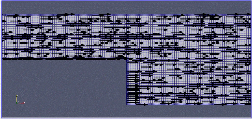
Velocity Vector near Recirulation:-
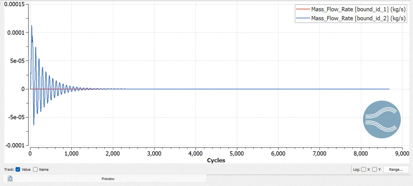
Mass_Flow_Rate Plot:-
Input and Output
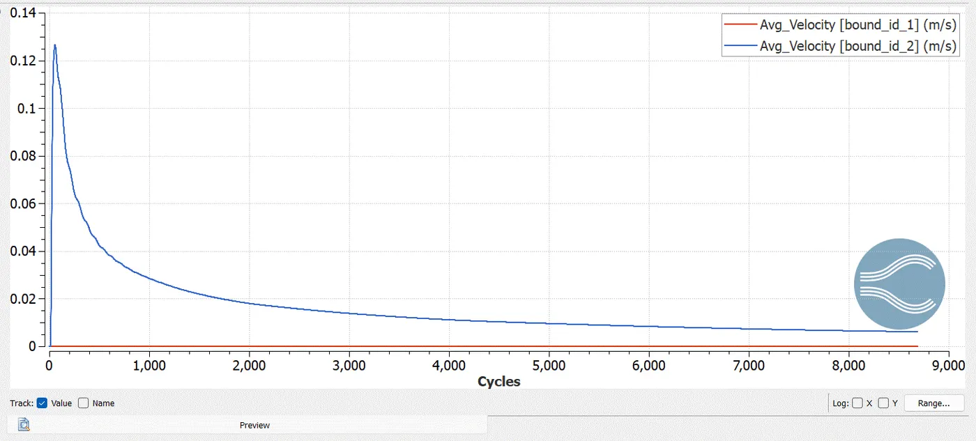
Velocity plot:-
Input and Output
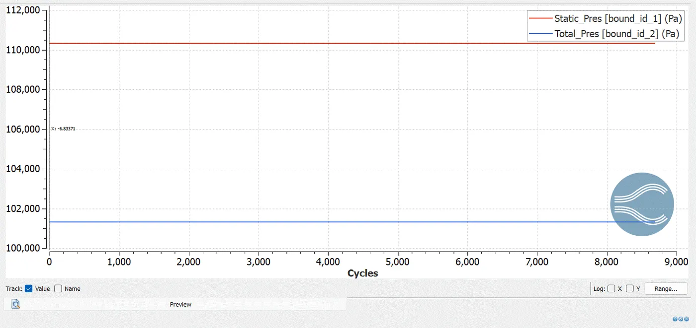
Pressures Plot:-
Inlet and Outlet
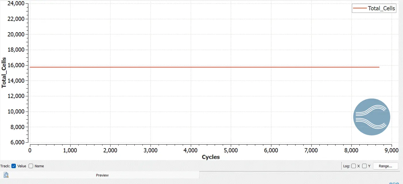
Total Cells Count's :-
Pressure Contour:-
Velocity Contour:-
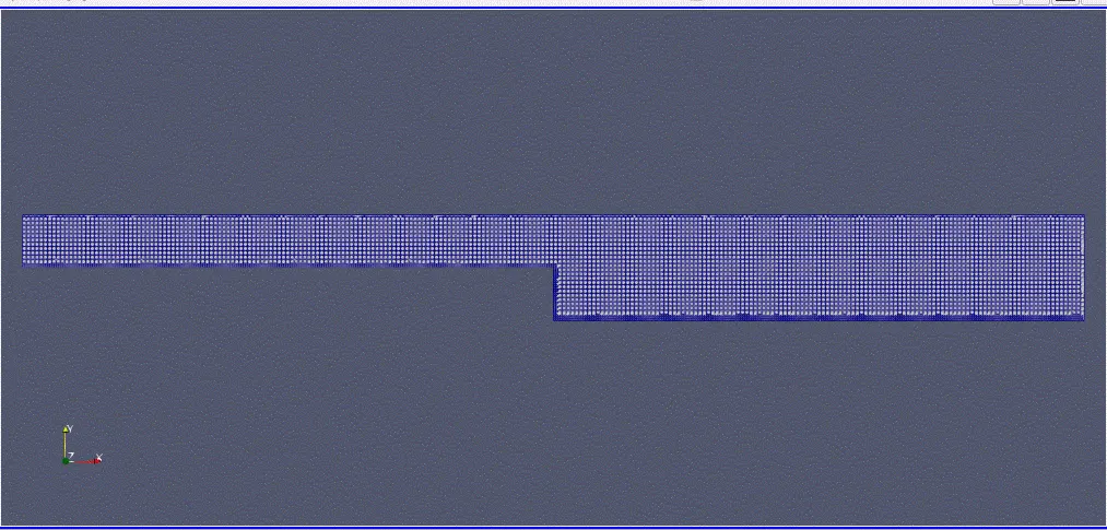
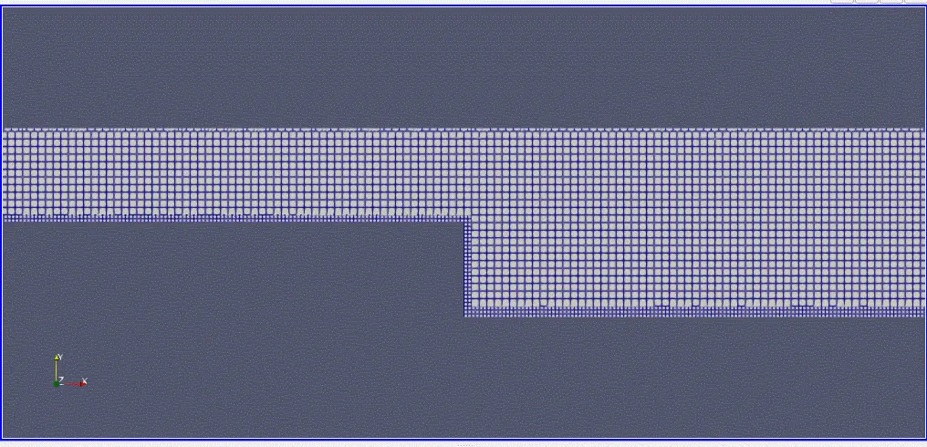
mesh grid:-
Case:- dx=1.0e-3m dy=1.0e-3m dy=1.0e-3m
NOTE:- change base grid size according to your setup
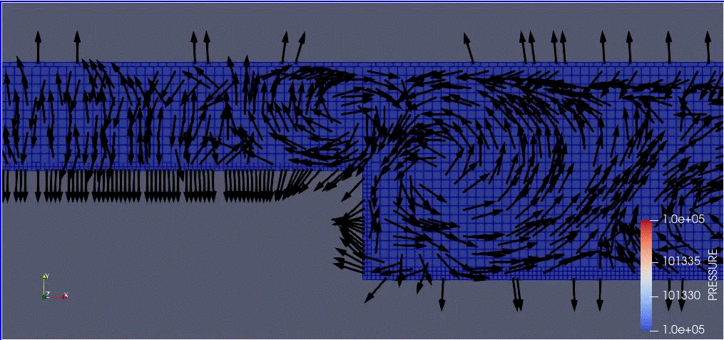
Velocity Vector near Recirulation:-
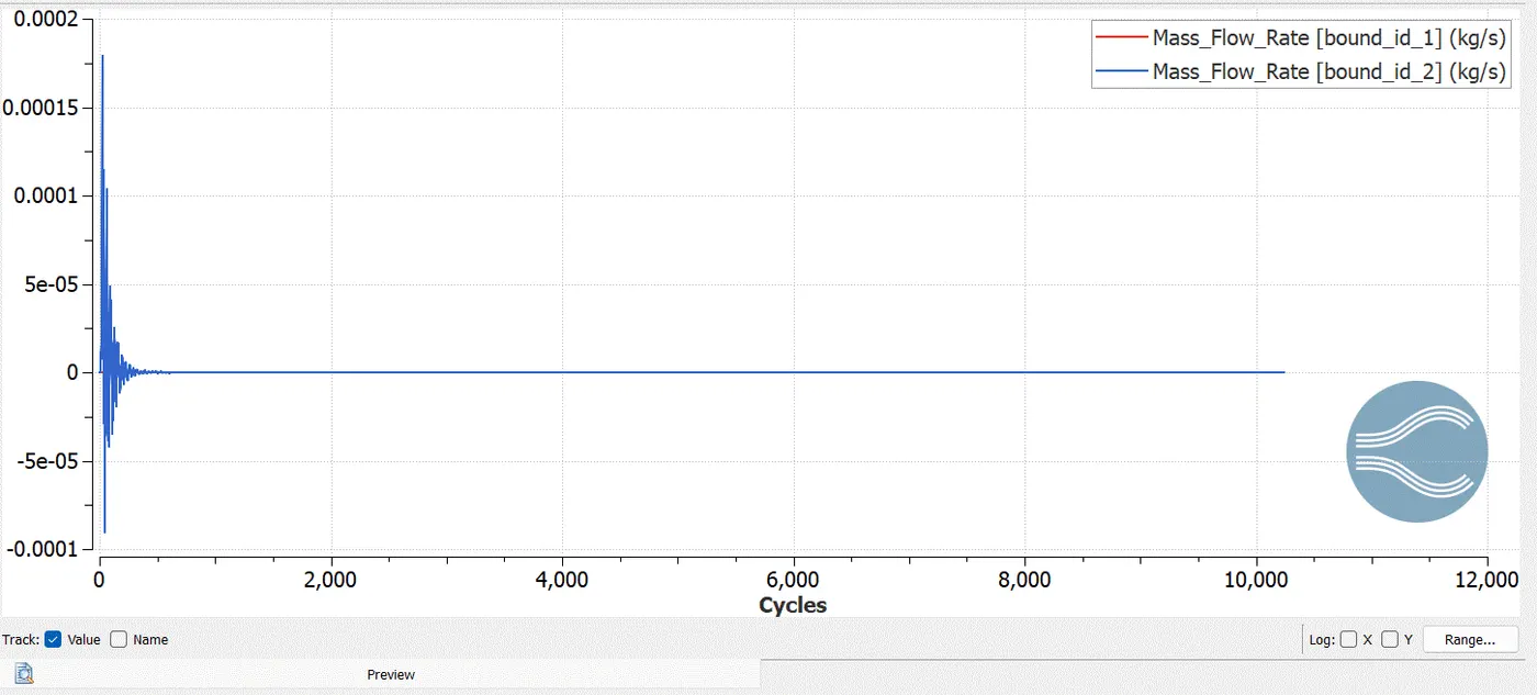
Mass_Flow_Rate Plot:-
Input and Output
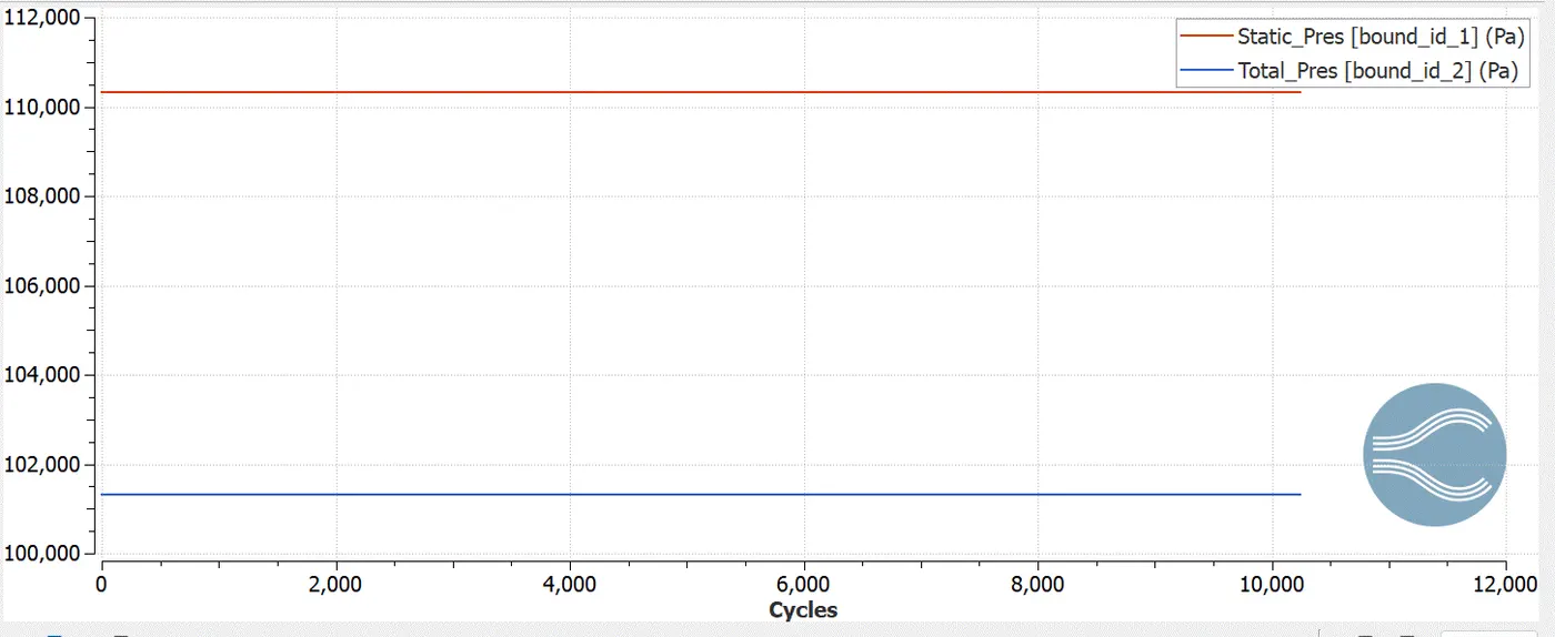
Pressures Plot:-
Inlet and Outlet
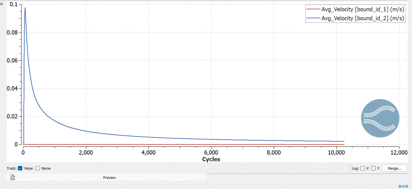
Velocity Plot:-
Inlet and Outlet
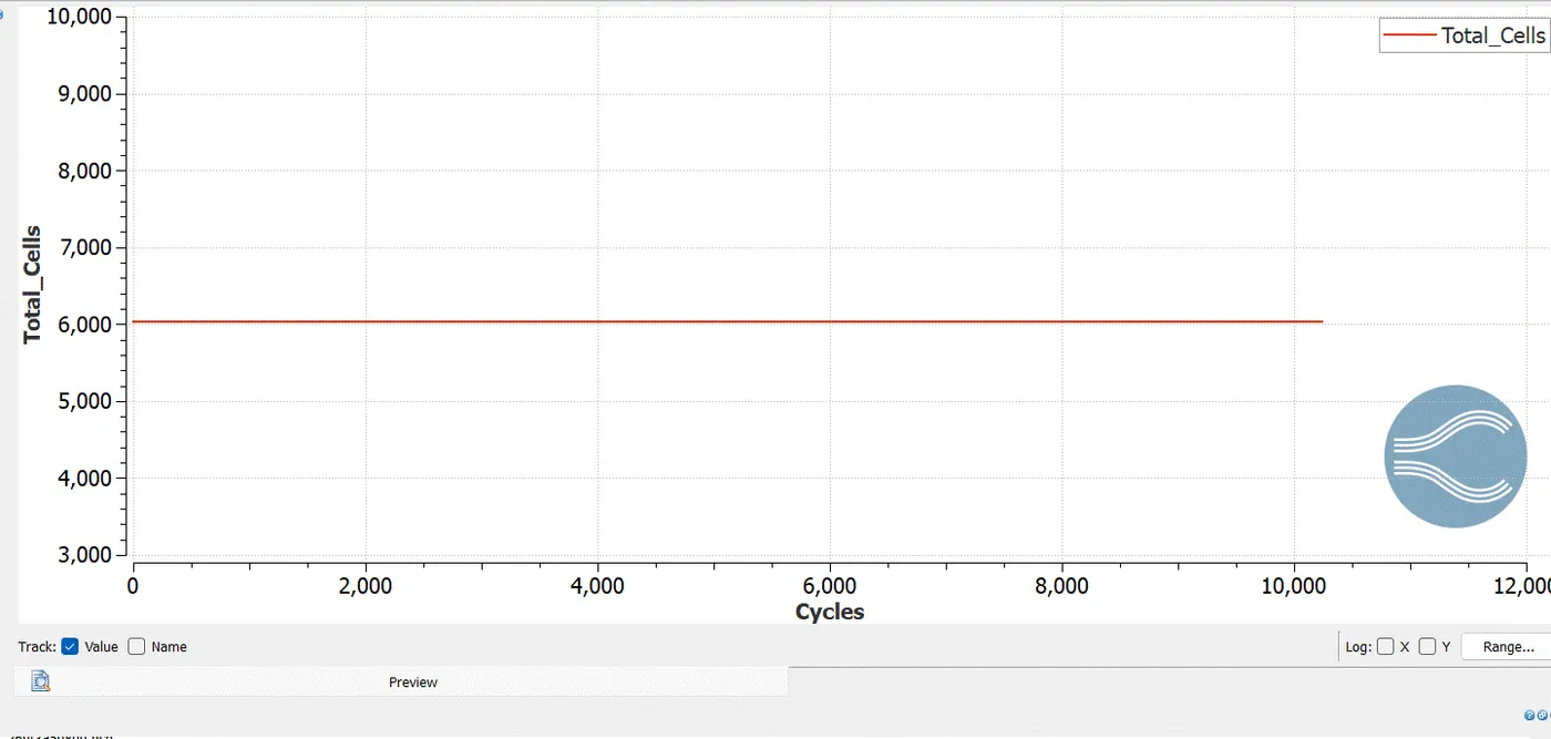
Total Cells Counts:-
Velocity Contour:-
pressure Contour:-