Week 3: Flow over a backward facing step

Aim:

To simulate flow through a backward facing step internal flow geometry using Converge with different mesh resolutions.

Theory:

Backward facing step geometry is a basic geometry that is preferred in the validation of turbulence models or their modifications. Various experimental results are available for this geometry which can be used to verify the compuational result. The separation and reattachment of flow over the step majorly depends on reynolds number of the flow and proper resolution of wall bounary layer. Hence the turbulence models chosen and mesh resolution play a major part in correctly predicting the reattachment point beyond the step. Generally k-omega SST model is preferred in these type of flows involving separation. In the current work though, the default turbulence model in Converge is used for demonstative purpose.

Case setup:

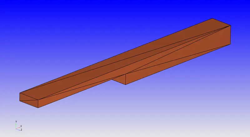
1. Import provided geometry in Converge studio. Enable the normal toggle and verify that the normals point to the inside of the geometry where fluid flow will occur. In the diagnostics dock, check if no issues are found with the provided geometry.

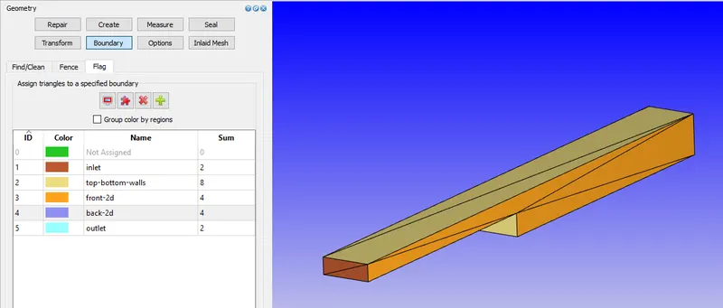
2. In boundary flag tab, assign each side of the boundary to a separe boundary. Rename the boundaries to represent their boundary type as shown in figure below

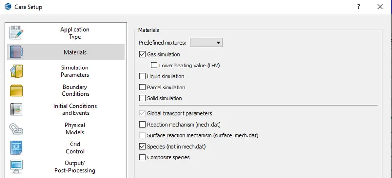
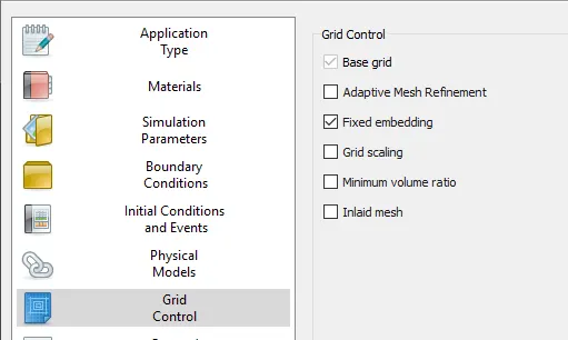
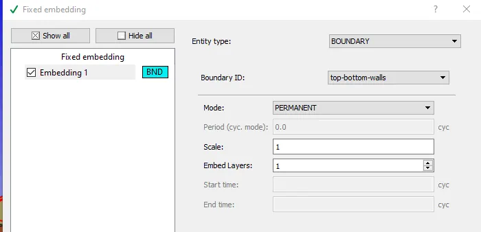
3. Open case setup, select application type as "Time based". Under Materials, select predefined mixture "air". Disable reaction mechanism and enable species. Under grid control, enable "fixed embedding" to increase mesh resolution near the wall. select ok to generate case setup tree.

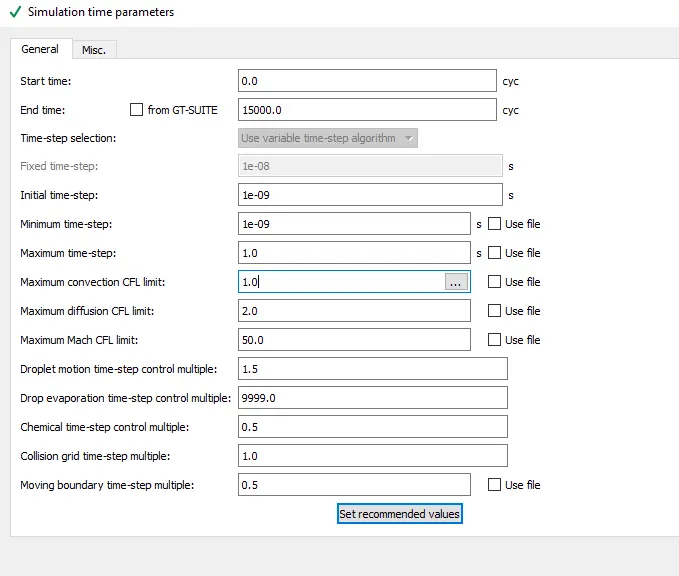
4. In run parameters, set solver type to "steady-state solver". In simulation time parameters, set end time to 15000 cycles and Time-step values as shown in figure below

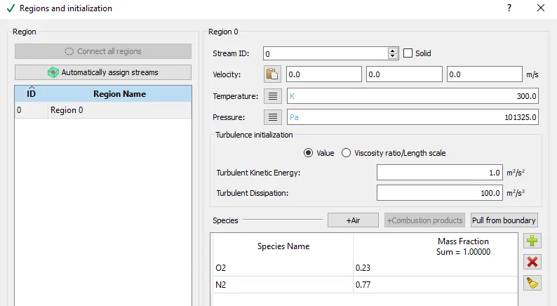
5. In regions and initialization tab, Add a region, set pressure value to 1 atm. Set species specificaiton to default air option. Use default value for other parameters and apply

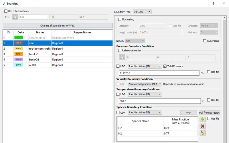
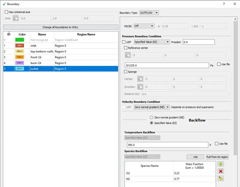
6. Set Boundary conditions for inlet as inflow with total pressure 111325 Pa, default temperature value and species mass fraction of air. Set outlet boundary as outflow with 1 atm static pressure and backflow species mass fraction of air. For wall use law of wall option for momentum and energy equations. Set back and front boundaries as 2D boundaries. Add "region 0" for region option for all boundaries

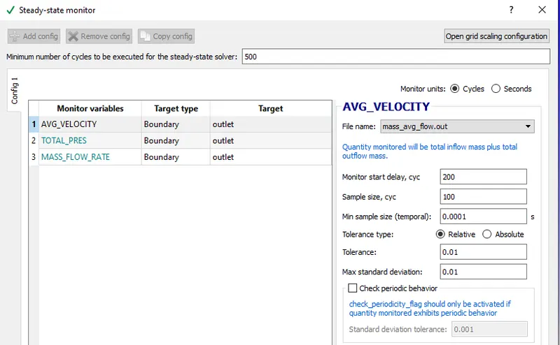
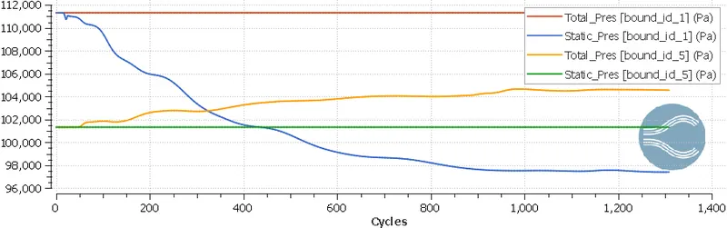
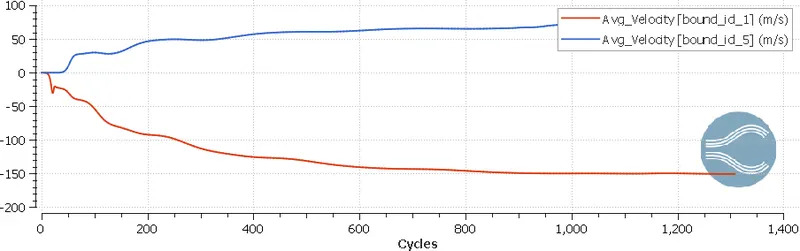
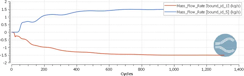
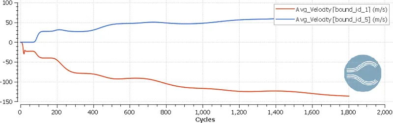
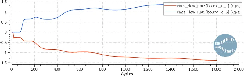
7. Add steady state monitors to check convergence of solution. Add monitors for average velocity, total pressure and mass flow rate at outlet.

8. Add O2 and N2 as species elements in species tab.

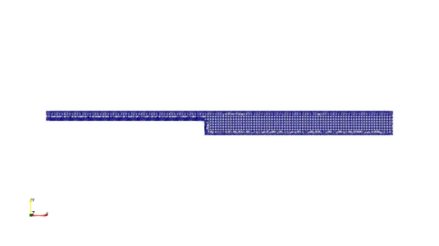
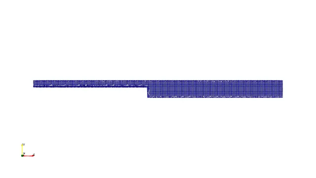
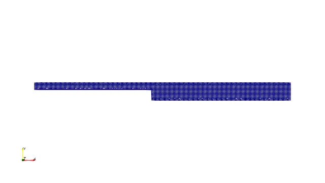
9. Generate 3 different cases with different base grid sizes as shown below

a. dx = dy = dz =2e-3m
b. dx = dy = dz =1.5e-3m
c. dx = dy = dz =1.2e-3m

10. For all the cases, set fixed embedding of scale 1 and embed layers 1.

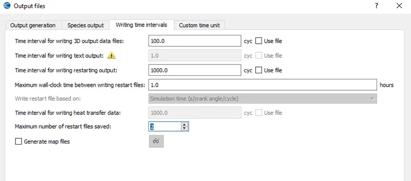
11. Set interval for writing output data to 100 cycles.

12. Export input files to a run folder. From cygwin run converge using msmpi using the input files for all the 3 cases

Results:

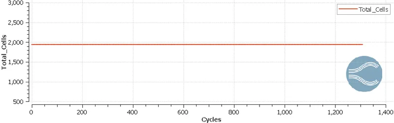
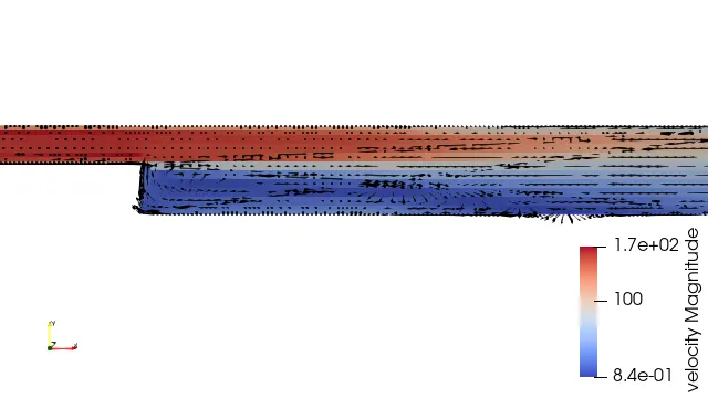
Case1:

Case2:

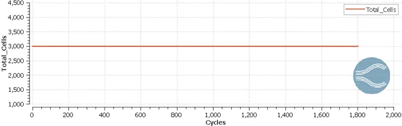
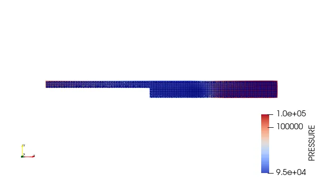
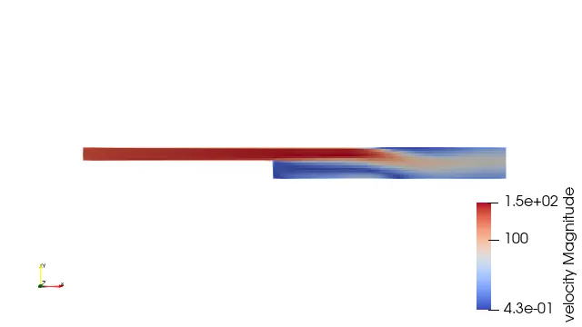
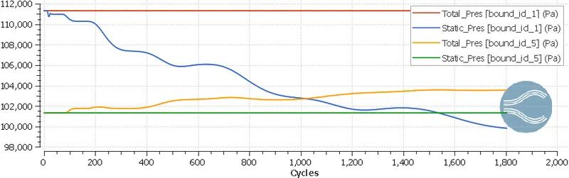
Case3:

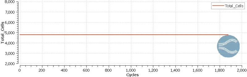
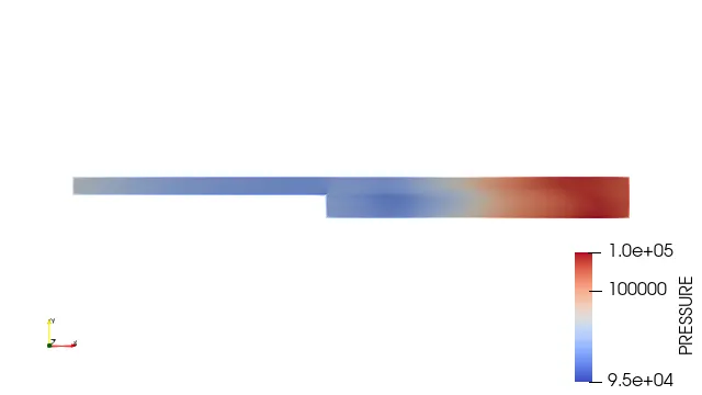
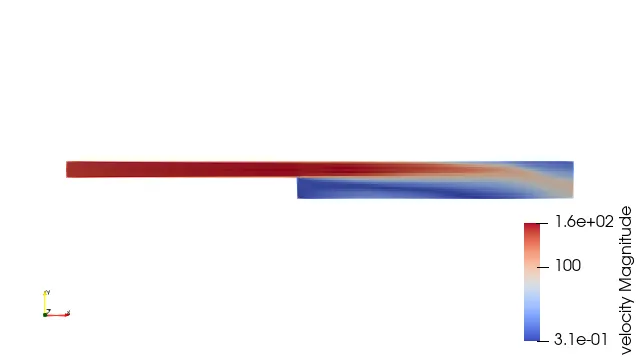
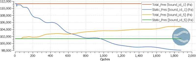
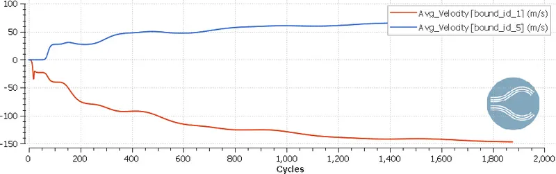
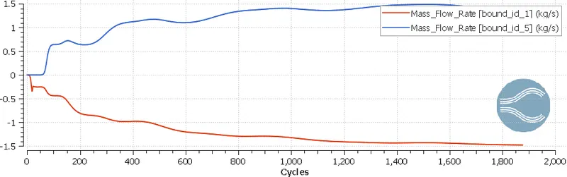
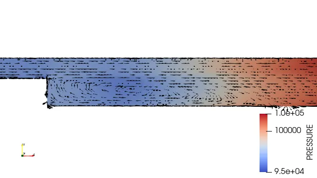
Conclusion:

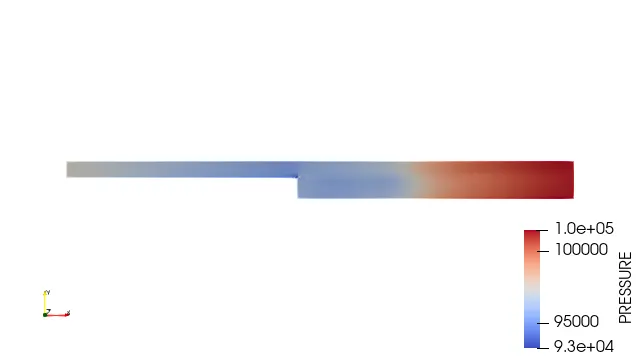
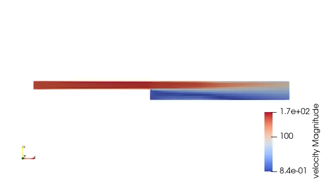
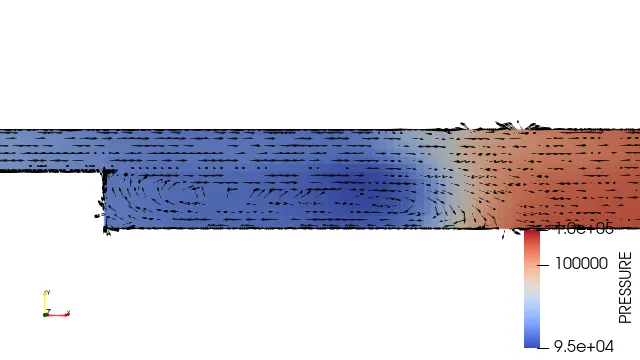
The contours and vectors show the flow profile in backward facing step geometry. All 3 meshes show expected flow behavior with recirculation region behind the step. With increase in mesh resolution, the velocity profile development in the domain seems better captured with less diffusion. However, it increases solution time by small margin. The size of recirculation zone and reattachment point prediction for each simulation can be compared with experimental result when available to quantitatively do the mesh independent study.