RESUBMITTING

Aim: Simulate the flow over the Ahmed body and use air as the working fluid with velocity of 25 m/s.

Objective :

• As the body is perfectly symmetric, we can run the simulation by considering the only half body. This is the best practice where you can save on the number of cells and get the results faster as well.
• The geometry which is provided with the challenge needs a modification which you should be able to do at this stage of a course. You need to use the 'split body' command in SpaceClaim to perform the operation and then you can use the symmetry boundary condition in fluent to perform the simulation.
• Run the simulation for the velocity of 25 m/sec with the default air properties in fluent.
• For this challenge, you will have to provide answers to the following questions:

Q1. Describe Ahmed's body and its importance.

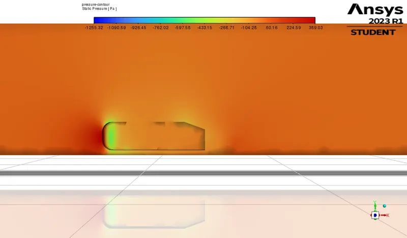
Q2. Explain the reason for the negative pressure in the wake region.

Q3. Explain the significance of the point of separation.

• Expected Results:

1. Velocity and pressure contours.
2. The drag coefficient plot for a refined case. ( For velocity of 25m/sec, the drag coefficient should be around 0.33).
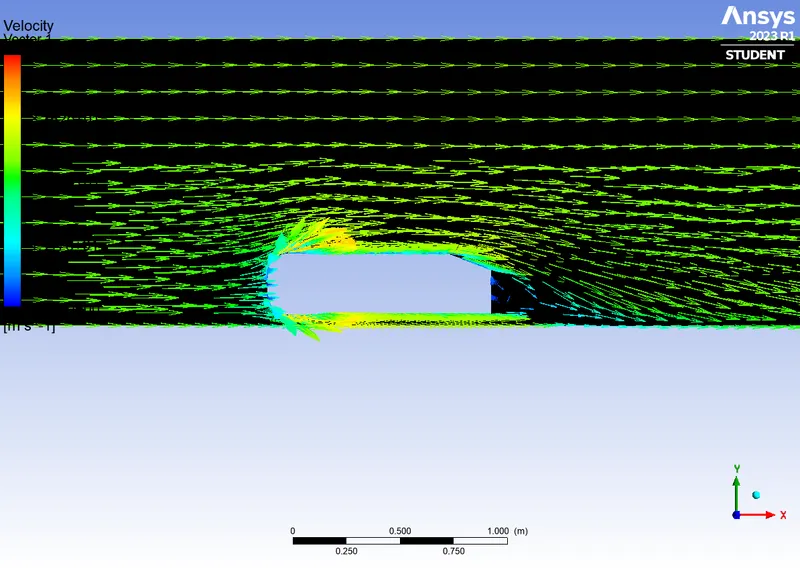
3. The vector plot clearly showing the wake region.
4. Perform the grid independency test and provide the values of drag and lift with each case.

Theory :

1. Reynolds number :

• The Reynolds number is a dimensionless number , named after the Osborne Reynolds , defined as the ratio of inertia forces to the viscous forces. Mathematically it is given as,

i.e. Re=ρVLμ��=ρ��μ

where ,

ρ = density of fluid (kg/m³)

V = velocity of fluid (m/s)

D = diameter of pipe (m)

μ = dynamic viscosity of fluid (N-s/m²)

ν = kinematic viscosity of fluid (m²/s)

• Significance :
  • Reynolds number is used in the forced convection. Forced convection is a type of heat transfer in which fluids are forced to move in order to increase the heat transfer.
  • Reynolds number is used to predict the flow patterns in the different fluid flow situation. At a low Reynolds number , the flow tends to be laminar flow, while at a high Reynolds number flow tends to be turbulent flow.

2. Type of flow :

• Laminar flow :
  • If a fluid travels smoothly in a regular path then flow is called as laminar flow. if flow is to be called laminar flow when the following conditions satisfy.
  • For internal flow, Re < 2000.
  • For external flow, Re < 10⁵.
• Turbulent flow :

• If a fluid flows in a irregular path instead of regular path, then it is called as turbulent flow. The flow to be called as turbulent flow when following conditions occurred.
• For internal flow, Re>4000
• For external flow, Re > 5 x 10⁵.

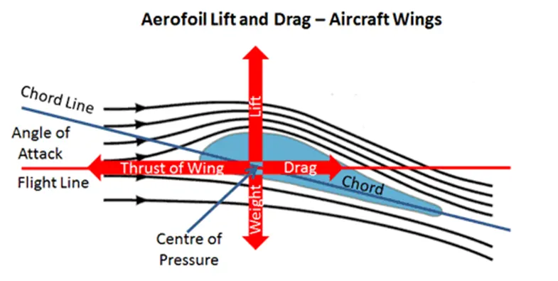
3. Lift and drag force :

1. When any body moves through a fluid , an intersection between the body and the fluid occurs and this effect can be described in terms of the forces at the fluid-body interface.
2. Both shear stress and pressure vary in magnitude and direction along the surface.
3. The resultant force in the direction of the upstream velocity is termed as Drag (D), and the resultant force normal to the upstream velocity is termed as Lift (L).

3.1. Drag Force(Fd) :

• Drag force is a resistance forced which is acting opposite to the motion of the object.
• It is mathematically given as

Drag force(Fd)=CdρAV22��ρ��22

Where ,

Cd = coefficient of drag

V = flow velocity

A = the projected area of the object w.r.t. which drag force is calculated.

ρ = density of fluid

• Drag coefficient is a dimensionless quantity used to determine the drag or resistance of an object in a fluid environment such as air ,water.

3.2. Lift force (F_l) :

• The force which is acting perpendicular to the object/body motion is called as lift force.
• It is mathematically given as

Lift force(Fl) =ClρAV22��ρ��22

Where,

Cl = coefficient of lift.

• Lift coefficient is a dimensionless quantity which is used to determine the lift of an object in a fluid environment such as air , water.

4. Flow separation :

• When a fluid is forced to flow over a curved surface at high velocities. A fluid follows the front portion of the curved surface with no problem but it has difficulty remain attached to the surface on the back side. At sufficiently high velocities, the fluid detaches itself from the surface of body. And this phenomenon is called as flow separation.
• The location of a separation point depends upon various factors such as Reynolds number, the surface roughness, the level of fluctuation in the free stream. And it is usually difficult to predict exactly where the separation will occurs unless there are sharp corners or abrupt changes in the shape of the solid surface.

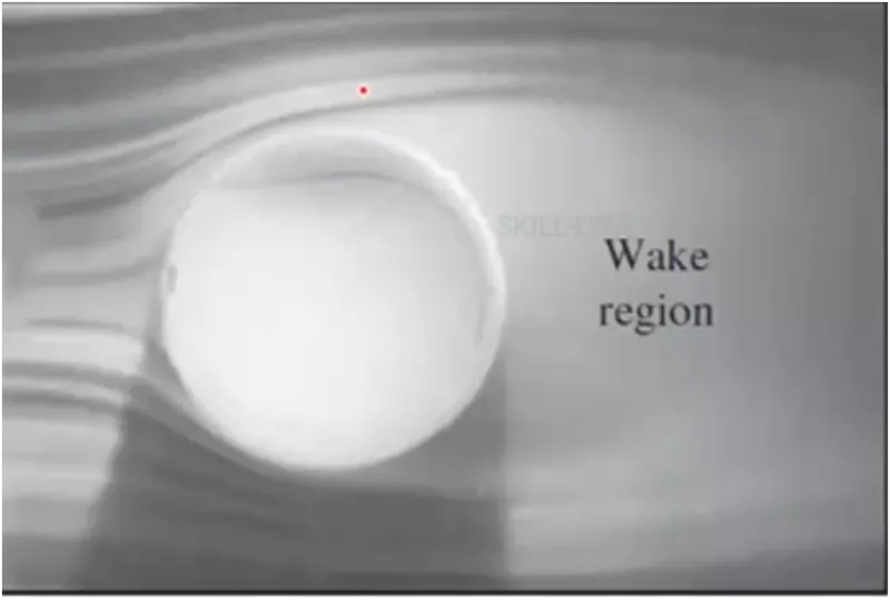
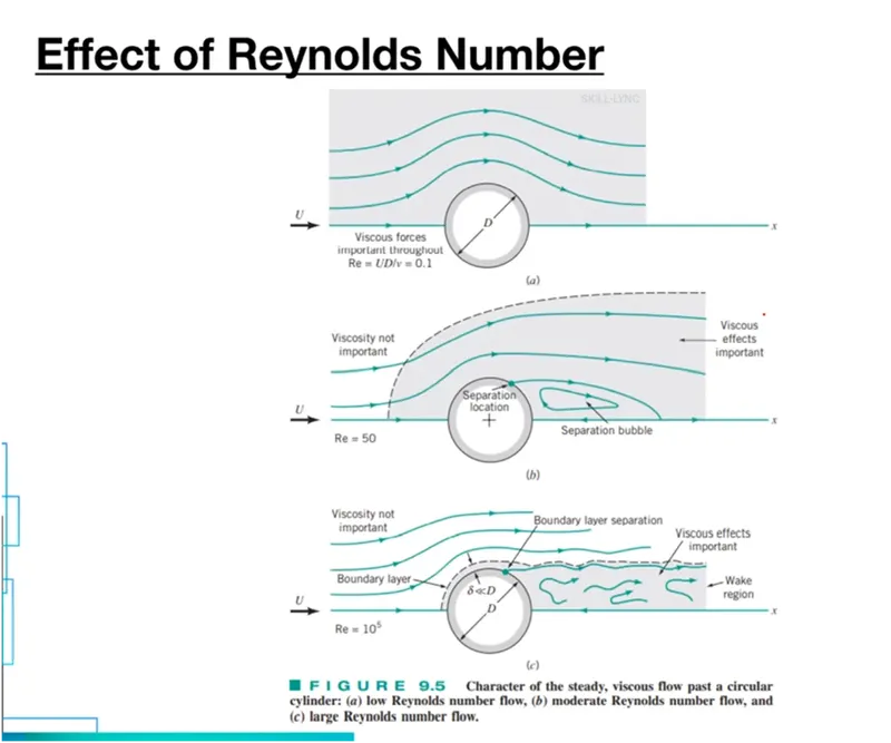
From above figure we can see that as Reynolds number increases the separation point moves towards left side and behind the cylinder wall the wake region increases.

5. Von-Karman vortex street :

• When the fluid flows towards the body, the flow around a bluff body produces a regular patterns of alternating vortices known as Von-Karman vortex street. The following figure shows Karman vortices visible in the clouds.

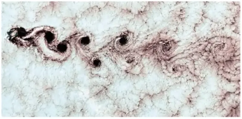
• These vortices produce a sinusoidal force acting on the body perpendicular to the flow. For a cylinder, the frequency (ωωin Hz) of the shedding is related to the diameter(D in m) and wind speed (V in m/s) given by Strouhal number(S)

S =ωDVω��

• Strouhal number (St) :

• In dimensional analysis, the Strouhal number (St) is a dimensionless number describing oscillating flow mechanisms.

6. Boundary layer concept :

• When any viscous flow flows over a surface, a region of slow-moving flow called boundary layer develops.
• Inside the boundary layer, there is a strong velocity gradient and U varies non-linearly.

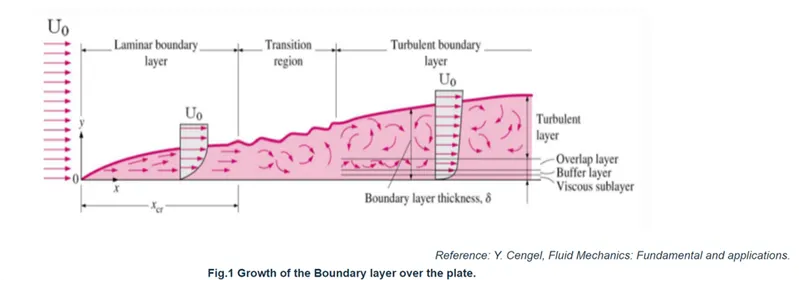
• The boundary layer comprises of –
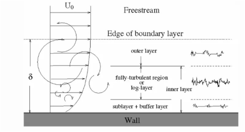
  • Inner layer i.e. 10-20% of total boundary layer thickness
  • Laminar sub-layer closest to the wall where viscous force dominates
  • Buffer layer where viscous and turbulent forces are of similar magnitude.
  • Log-law layer where turbulent forces dominates and velocity exhibits logarithmic variation.
  • Outer layer (law of the wake) where inertia forces dominates and flow is free from viscous effects.

7. Y-plus :

• The behaviour of the flow near to the wall is a complicated phenomenon and to distinguish the different regions near the wall the concept of wall has been formulated and this concept is called as y-plus. Thus it is a dimensionless quantity and is measured in terms of viscous lengths.
• To resolve the effects near the wall i.e. the viscous sublayer, the size of the mesh size should be small and dense enough near the wall so that almost all the effects are captured. But in some cases, if the wall effects are negligible then there is an option of including semi-empirical formulae to bridge between the viscosity affected region and fully turbulent region , and in this case , the mesh need not be small or dense near the wall i.e. course mesh required.
• Considering the first case, i.e. near wall modelling it is well known that the small size mesh is required but the question arises that how much small size mesh required? Thus, here the concept y⁺ comes into picture and based upon the Y-plus value the first cell height can be calculated. The near wall region is meshed using calculated first cell height with gradual growth in the mesh so that the effects can be captured and avoids large mesh cell counts.
• The boundary layer components can be distinguished as follows
  • Laminar sublayer : Y+ < 5
  • Buffer layer : 5< Y+ < 30
  • Log-law layer : 30 < Y+ < 300
• Some turbulent models resolve laminar sublayer while others model it. therefore it is important to place the first cell centroid in either laminar sublayer or lag-law layer acoordingly.
• For a CFD simulation, we can compute the first layer height for a desired Y+ value as

y=y+μρu∗�=�+μρ�∗

where,

u∗=τwρ�∗=τ�ρ

τw=12⋅CfρU∞2τ�=12⋅��ρ�∞2

Cf=0.0576Re−15��=0.0576��-15

Re=ρU∞Lμ��=ρ�∞�μ

Where,

y= first cell height

μ= viscosity

ρ = density of fluid

u_* = frictional velocity

τ_w = wall shear stress

C_f = skin friction coefficient

U_∞ = free stream velocity

L = boundary sublayer thickness

8. Inflation layers :

• To capture the viscous effects near the wall we need small mesh size. to resolve the gradients, the cells need to be smaller normal to the wall than along the wall.

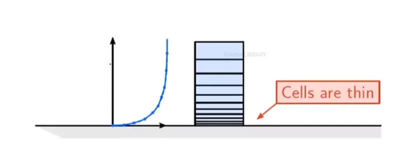
• Real geometries are complex and we often need to use an unstructured mesh. But the unstructured mesh are not thin enough close to the wall. so we can grow prism layers under beneath the unstructured mesh to provide the thin cells that we need to resolve the gradients. And these prism layers are called as inflation layers.

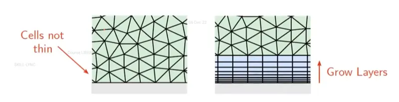
• It is common aim for the boundary layer thickness(δ₉₉) to be contained within the inflation layers. Hence, we need to formula to calculate the total height of the inflation layers. Then we can ensure that δ₉₉ is within the inflation layer.

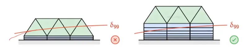
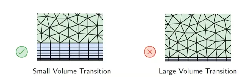
• There should be good volume transition required.

8. Ahmed body :

• Ahmed body is nothing but a car model which uses to simulate the CFD results and validates with the actual results.
• The results like drag coe. , lift coe. , pressure, velocity etc. for different car models and compare these results with ahmed body results.
• Optimized external car aerodynamics is necessary to achieve efficient vehicles with minimized fuel consumption, CO2 emissions, and noise, while keeping a good driving stability. Steadily increasing computer power has been raising the importance of simulating the external aerodynamics of vehicles and computing the corresponding aerodynamic characteristic numbers. At present, an efficient resource management gains increased importance everywhere. A substantial part of the development time of cars is therefore invested in optimization. This is possible only and particularly by virtual development. In order to establish such development processes in the car industry, reliable simulation models validated by experiments are needed.
• Model experiments suitable for providing validation data make use of model bodies with geometries characterized by variable parameters, such as the slant angle at the back. One such body is the Ahmed body, a bluff model body of simple shape with basic aerodynamic properties of a vehicle, which has been used for many reference investigations.

9. The reason for the negative pressure in the wake region:

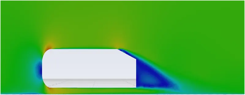
• As the high velocity fluid strikes on the frontal side of body due to this the velocity gets reduced and pressure increases. But as body moves the fluid is attached to the body and it moves forward. But when the fluid leaves the body due to sudden change in dimensions or sharp corners the flow separation occurs and behind the body there is low velocity region creates and this region is called as wake region.
• In this region the eddies are formed and due to these eddies a vacuum creates. It means the negative pressure creates. It means there is no fluid element present. Due to absent of fluid molecules in wake region some negative pressure creates.
• Due to this negative pressure some pulling force observes in wake region. Also we experience a lift force.
• Also this wake region there is more turbulence occurs due abrupt changes.
• As the velocity increases the point of separation moves left side and the wake region area reduces but still there is negative pressure or vacuum remains.
• We can clearly understand this concept further by looking contour plots.

10.Mesh(grid) independent study :

• It is a method of investing, whether the simulation results are independent of the underlying mesh or not.
• For that first of all we will start with the course mesh size and finding out the reasonably accurate results.
• After that we are refining the mesh size i.e. decreasing the mesh size and run the problem for several times until achieving almost constant results such as drag, lift, temp, heat transfer coe.’s in case of fluids, heat analysis etc.
• After finding out the results we will compare these results with previous solutions and then Find out the optimum grid/mesh size condition that has the smallest number of grids without generating a difference in the numerical results.

Modelling approach :

1. Pre-processing method :

1.1. Geometry cleanup :

• Open workbench.
• Drag fluid flow(fluent) to the project scheme.
• Firstly import the cad file to the geometry.
• Then right click on geometry -> edit geometry in space-claim.

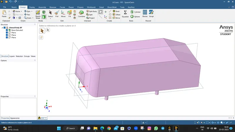
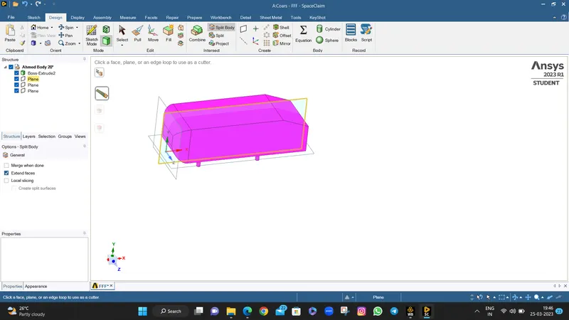
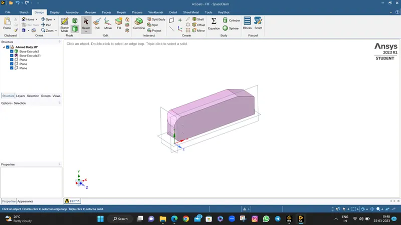
• Now, this is the symmetric car model. so lets delete the half portion of a body. For that first of all creates plane and use split body tool under design to split the body along the plane. Then hide the planes.

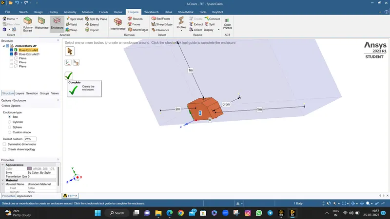
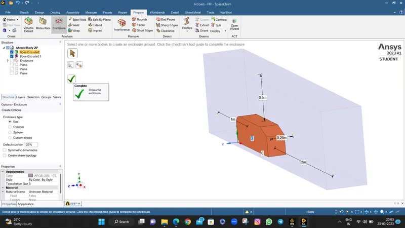
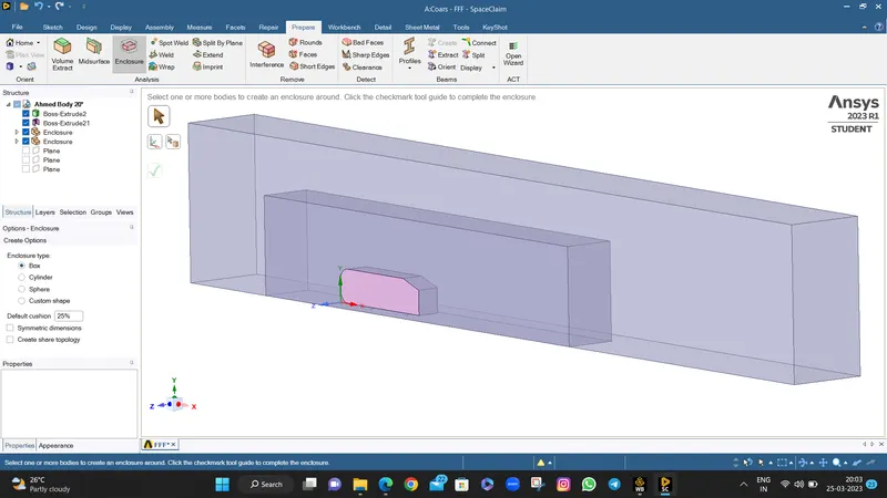
• Now, lets create the fluid domain around this car model. For that we are creating 2 enclosures with standard dimensions.
• To create enclosure goto prepare -> enclosure -> select body -> uncheck symmetric dimensions under outline -> give appropriate dimensions. -> click on green tick.

• Lets see sectional view.

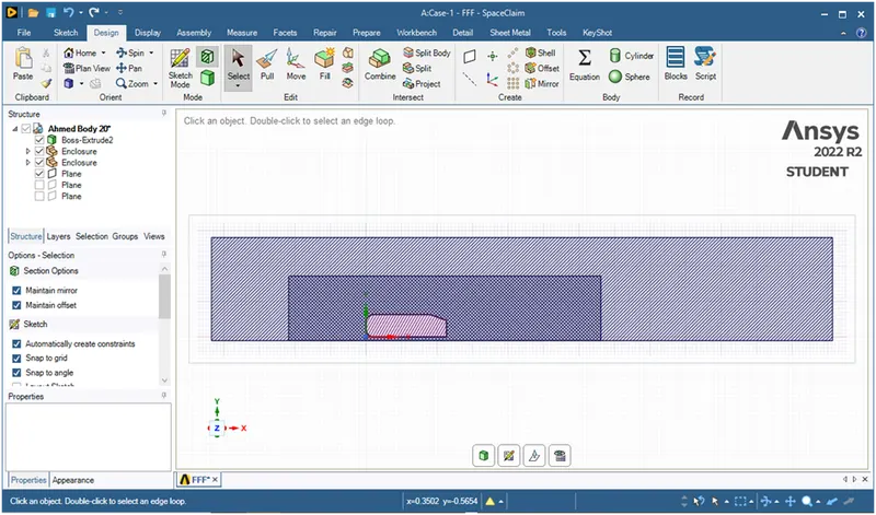
• Now the some common area is represented by looking hatches which are overlaps. So delete this common area by using interference tool under prepare.

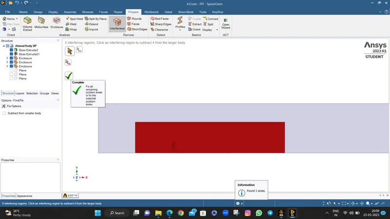
Now this common area has been removed.

• Let’s enabled share topology to share the information between two enclosures through common node points. Before enabling share topology just suppress the car model for physics.
• To enabling share topology goto workbench and enabled share by selecting geometry.

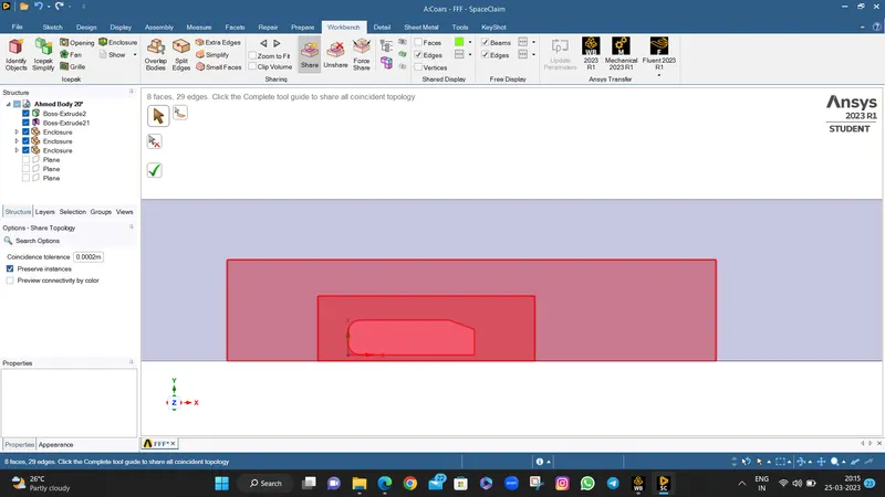
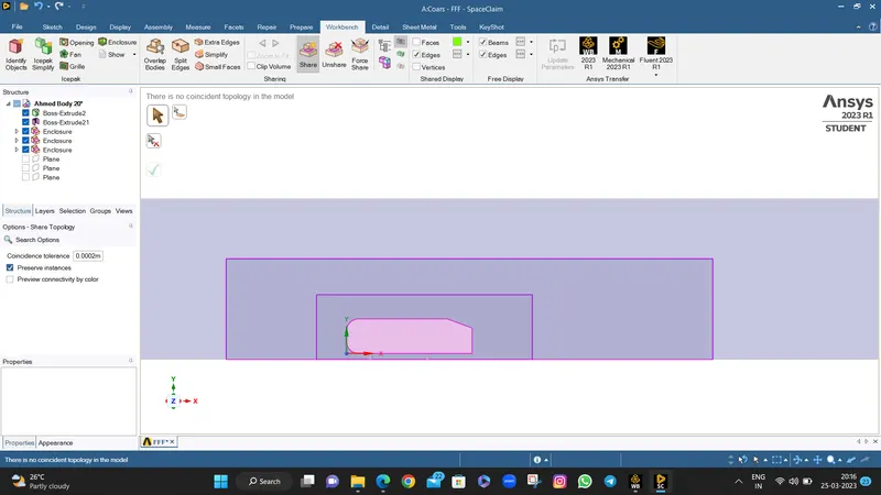
Now, its done.

1.2. Meshing :

• Open mesh.

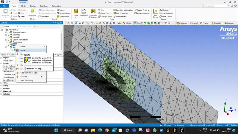
• Select the faces and gives the name as shown below

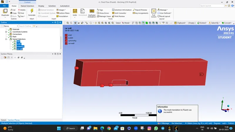
• Now we will create the course mesh on outside enclosure and fine mesh on inner enclosure.
• Here we are doing mesh independent study to finalize the mesh size by comparing the results for different sizes.
• Lets create the multizone mesh for outer enclosure.
• Then create face meshing for inner enclosure.
• Then creates an inflation layer around the car wall to capture the viscous effects near the wall.

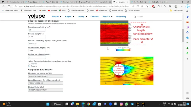
• First we will calculate the first layer thickness.

For that we put free stream

velocity = 25 m/sec

Characteristic length = 1.004 m

Desired Y+ = 5

So, We have First Layer Thichness = 0.074385 mm

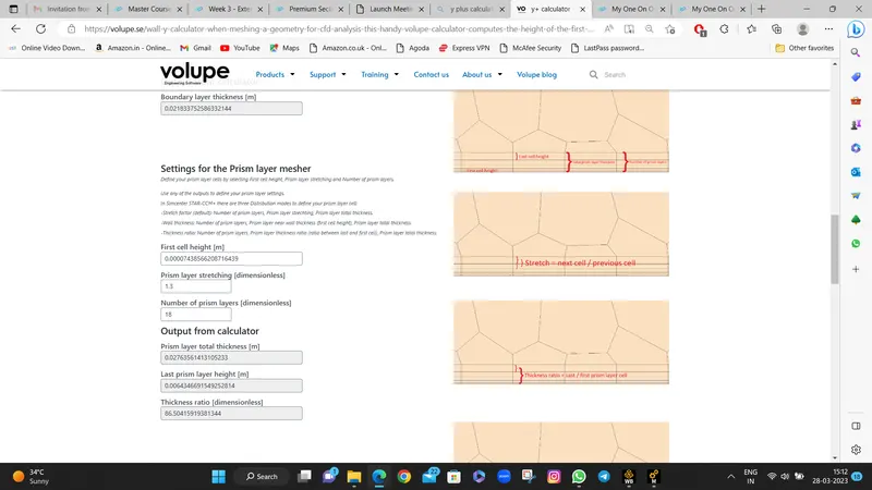
Growth Factor = 1.3

No. of layer = 18

So we got prism layer thickness = 0.027635.

which is greater than Boundary layer thickness.

• In above First inclosure We have 100 mm mesh

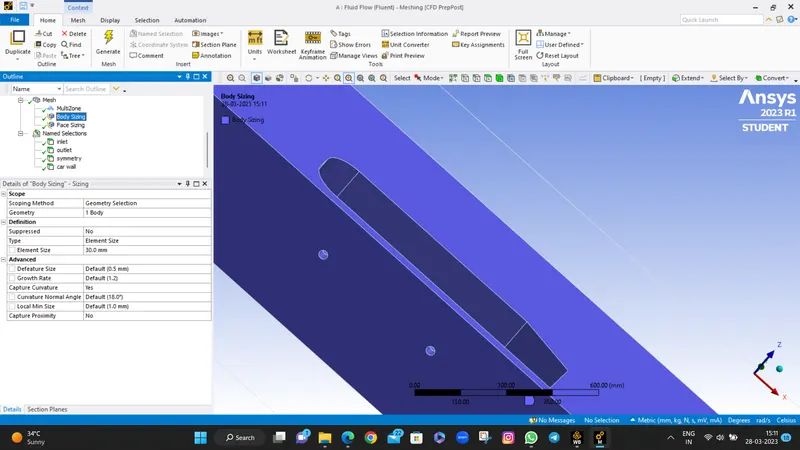
• In above for body sizing 30 mm mesh size

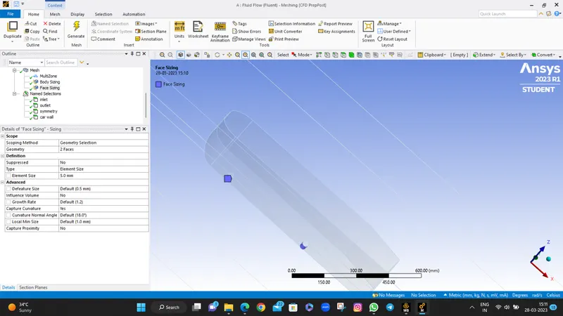
• In face sizing 3 mm mesh

• In inflation layer
• First layer height = 0.0744
• max layer = 18
• Growth rate =1.3

Total Elements = 488243

2. Post-processing method :

• Open the setup

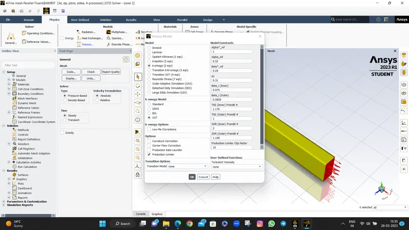
• Apply following conditions.

Solver	Pressure based
Time	Steady state
Model	K-ε-standard-enhanced wall fn
Material	Air (ρ=1.225kg/m3 , µ= 1.7894e-05 Pa-s)
Boundary conditions	Inlet- V=25m/s

• Now change the reference values as shown below

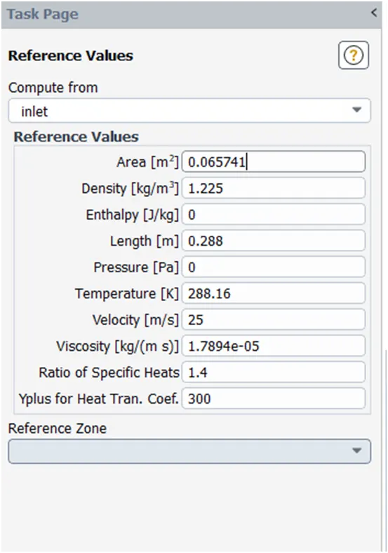
• Now creates 2 new report definitions as drag and lift.
• Initialize the solution
• Run the simulation for some 600 iterations.

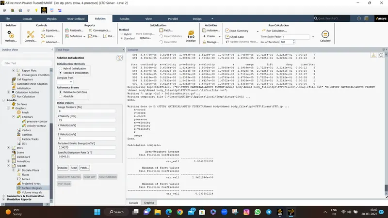
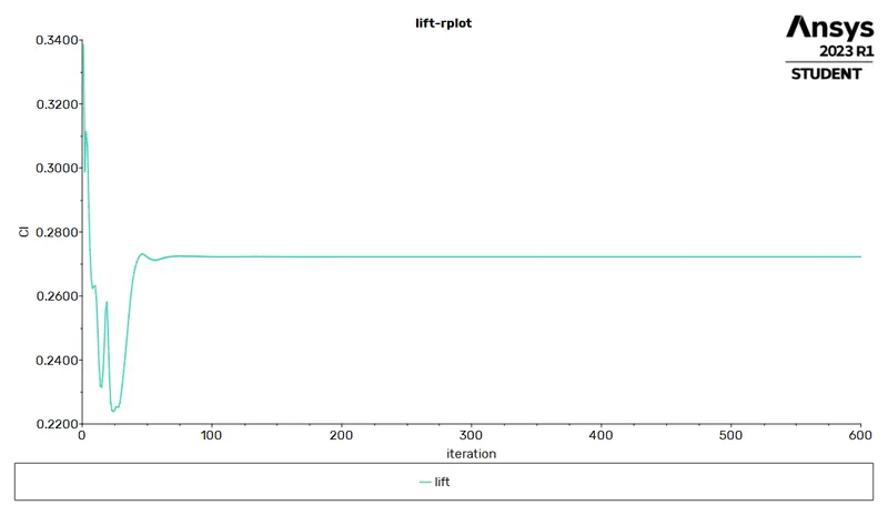
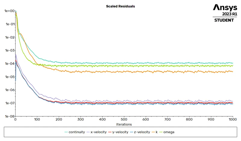
Now solution has been converged.

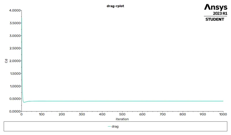
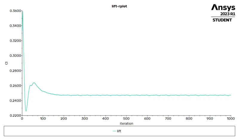
• Now saved the residual,drag,lift plots.

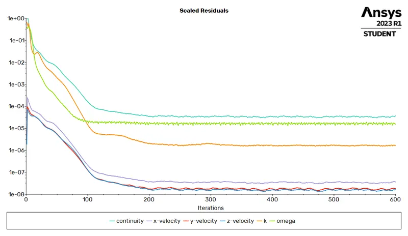
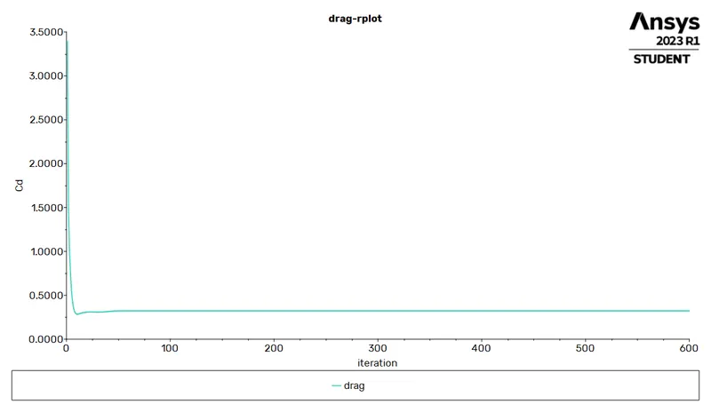
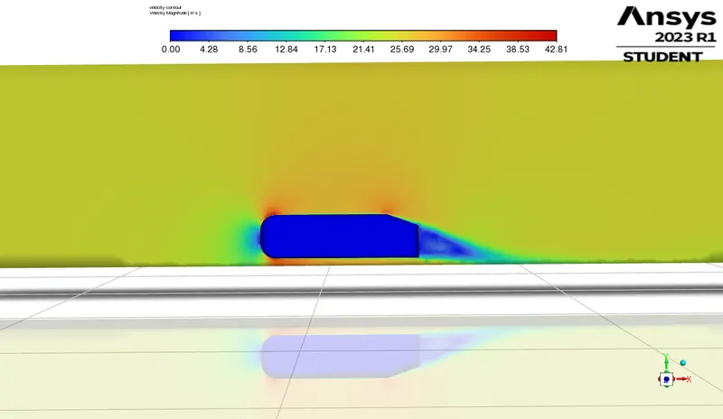
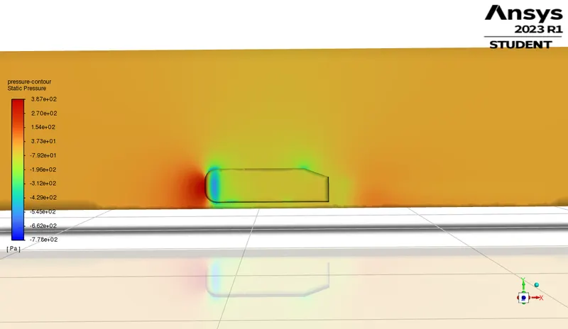
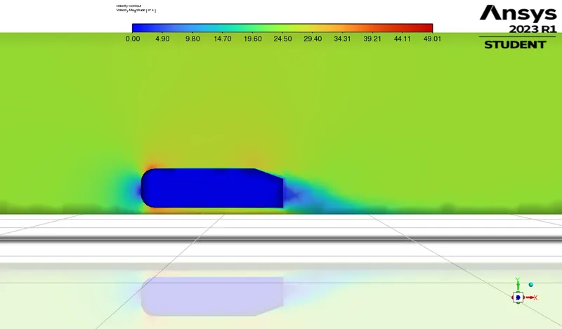
Now open the cfd-post and plots a velocity, pressure contour plots and also velocity vector plots. And saved these plots.

For that firstly create the xy-plane and then creates the contours

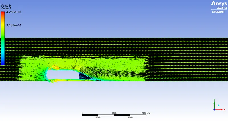
• Now repeat total procedure by changing the mesh size i.e. by Coarse mesh grids and find out the drag,lift, contour plots.

Results :

• Grid independent study

Cases	Mesh types	Cell counts	Drag(Cd)	Lift(Cl)
1	Fine mesh	488243	0.3226	0.2722
2	Coarse mesh	66480	0.4050	0.2470

• Residual plots

Cases

Plots

1.

2.

• Drag plots

Cases	Plots
1
2

• Lift plots

Cases	Plots
1
2

• Velocity contour plots

Cases	Plots
1
2

• Pressure contour plots

Cases	Plots
1
2

• Velocity vector plots

Cases	Plots
1
2

Conclusions :

• From mesh independent study we can say that, the drag coe. (C_d) =0.40 considered as there is student licence restriction we can’t increase the total number of cell counts beyond 5,12,000. And by refining the mesh quality we can see the drag also drops but gets an avg value and by comparing this with actual results that gives drag around 0.32. so we can say that our results are validates.
• By seeing drag plots, lift plots and residual plots we can conclude that , the solution has converged. Here the convergence means after the certain iteration done we are getting constant graph plots and gets constant values.
• From velocity contour plots and pressure contour plots we can say that, as we are refining the mesh quality the contour plots also gets more deviated i.e. we can see more clearly how velocity and pressure distributes in a fluid domain over a model as going forward w.r.t. length.
• From velocity contour we can say that, as air moves in fluid domain with 25 m/s velocity uniformly but when the air strikes the frontal portion and due to this there is a sudden drop in a velocity magnitude. And this kinetic energy converts in pressure energy. Now, due to strike, air flow changes the path and moves over a surface and near the wall the velocity remains low due to resistance or wall shear effect or max well condition at boundary.
• Now, behind the ahmed body we can see that a some low velocity region has been created for certain length. This low velocity region is called as wake region. And in this region a vacuum created i.e. low presuure/negative pressure region . This is because as previously this space is taken by car but as the car moves forward so there is an empty space created.
• And also due to sudden change in the geometry or due to sharp corners there is a flow separation occurs at a certain point. And this point is called as point of separation. There is huge importance of this point. The parameters like, flow separation, turbulence created in fluid, lift force etc depends upon this point. As velocity of fluid or velocity of car which moves in air ,this point of separation moves opposite to the fluid flow direction and the flow separation reduces. Also drag reduces.
• From pressure contour plot we can say that, there is a sudden increase in pressure at frontal portion of a car model. Now this is due to the high velocity fluid strikes on the frontal wall of car. Due to this the velocity reduced but the net energy remains same according to 1^st law of thermodynamics and according to Bernoulli’s principle the total energy is a summation of pressure energy, kinetic energy and potential energy is remains constant by assuming there is no frictional head loss and here the potential energy is constant so this kinetic energy converts into pressure energy and here the static pressure increase.
• Now from vector velocity plot we can clearly see that the how the wake region has formed. Also how the fluid moves over a body and variation in the velocity of air over a body. Also we can see that how the flow separation occurs.

Reference papers :

1) Flow and Turbulence Structures in the Wake of a Simplified Car Model

2) Experiments and numerical simulations on the aerodynamics of the Ahmed body