Week 3 - External flow simulation over an Ahmed body.
AIM:
To perform the flow study over a Ahmed's body and to study the behaviour of the fluid flow. To perform the grid independency test to analyse the accuracy of the result and to improve it. To understand basic concepts of how the fluid flow over a body creates the drag force in it. To understand the concepts of point of seperation, wake, vortices occured during the simulations.
THEORY:
Need for the Ahmed Body:
The drag coefficient quantifies the resistance of an object in a fluid environment. It is not an absolute constant and varies with the shape & size of the body and speed & direction of the flow. The lower the drag coefficient, less will be the aerodynamic and hydrodynamic drag occurs.
With that consideration, we are not supposed to reduce the drag force drastically as it will lead to the reduced downforce and leads to the reduced road friction. So identifying the drag force is the crucial work for the engineers. Because with the increased drag force, fuel efficiency will reduced and the power consumption is also increased. So as the industry electrifies, we have to make much focus on reducing the unwanted forces that reduces our valuable source of energy.
A major contribution of drag in the vehicle is the pressure drag. A key feature of flow field around a vehicle are the region of seperated flow. Even a simple basic vehicle configurations wil smooth surface generates varieties of Quasi-Two dimensional and fully three dimensional regions of seperated flows. So with this consideration S.R. Ahmed creates simple geometry to study the features of flow seperated region & wake. Such Geometry is called as Ahmed Body.
Ahmed Body:
Ahmed body is a benchmark model widely used in automotive industry for validating simulation tools. It is simple shape enough to model, while maintaining car like geometric features.
Considerations of Ahmed Body:
Selection of the configuration used in this study has governed by the requirement that it should generate essential feature of the real vehicle flow field with the exemption of that due to rotating wheels, engine and passenger compartment floor, rough underside and surface projections. It is assumed that the model should generate
- a strong three-dimensional displacement flow in front.
- relatively uniform flow in the middle
- large structured wake at the rear.
INTRODUCTION:
We are going to analyse the flow study over a Ahmed's Body in the following cases
CASE I: Random Meshing(Automatic Meshing)
CASE II: Meshing Refinement - Outer Enclosure = 75mm; Inner Enclosure = 40mm; First Layer Thickness = 3mm.
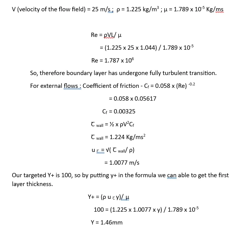
CASE III: Meshing Refinement - Outer Enclosure = 58mm; Inner Enclosure = 36mm; First Layer Thickness = 1.46mm.
PROCEDURE:
Geometry Study:
Understanding about the basic geometry provided before going for the simulation is the important one. The basic dimensions of the ahmed body remains the same. As we all know from the many research paper published in previous the wake, vorticity behind the ahmed body varies with reference to the slant angle provided at the end of the ahmed body. The provided geometry has slant angle 20 degree, which we have to consider for choosing the method to solve the geometry and the parameters to be used.
Here in this image we can be able to see how the vortices changed with respect to the slant angle provided at the rear end of the ahmed body.
Domain Used:
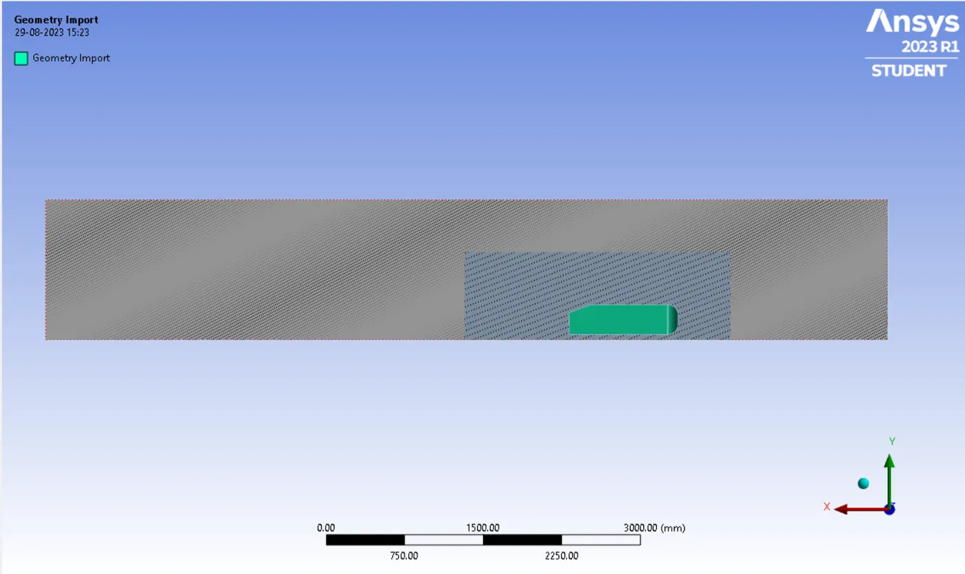
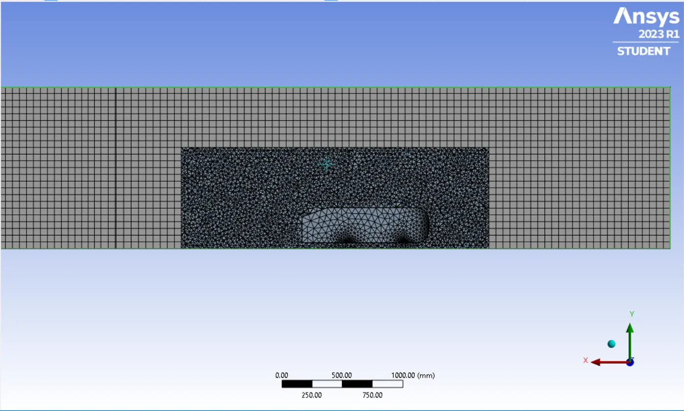
After the understanding about the geometry, then we have to set up the domain for running our simulation. Normally the race modeled cars are tested in a wind tunnel conventionally, whereas it take lot of resources. In order to eliminate that we are using that model of the wind tunnel in our CFD software to recreate the similar details. For our geometry the wind tunnel created are as follows,

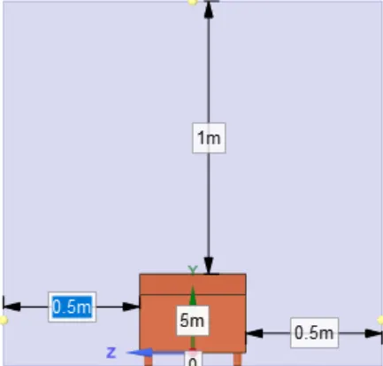
Here for achieving the better results we are provided the additional boundary (Refined boundary) which is closer to the model.
Meshing :
Now we can mesh the geometry. As we already discussed we will mesh the geometry considering the three cases, as our aim is to study the simulation of fluid over an ahmed body.
CASE I: Random Meshing (Automatic Meshing)
CASE II: Meshing Refinement - Outer Enclosure = 75mm; Inner Enclosure = 40mm; First Layer Thickness = 3mm.
CASE III: Meshing Refinement - Outer Enclosure = 58mm; Inner Enclosure = 36mm; First Layer Thickness = 1.46mm.
CASE - I:
Imported the geometry and do the Automatic meshing, where Ansys preferred meshing model to us.
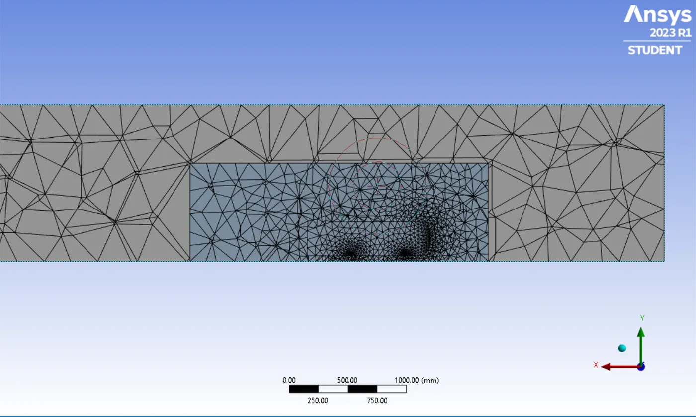
CASE - II:
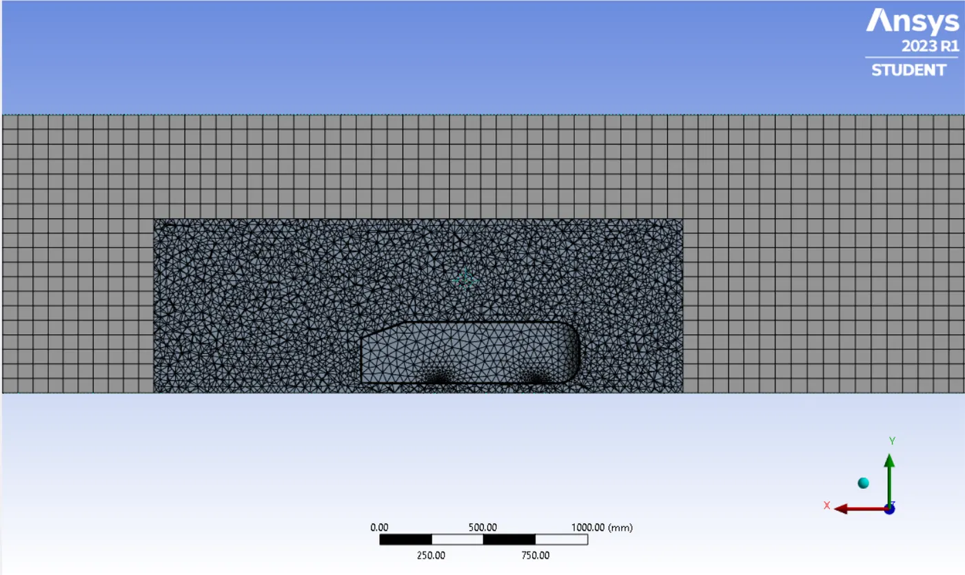
Outer Enclosure - Multi Zone Method - 75mm
Inner Enclosure - Element size - 40mm
Inflation Layer - First Layer Thickness - 3mm
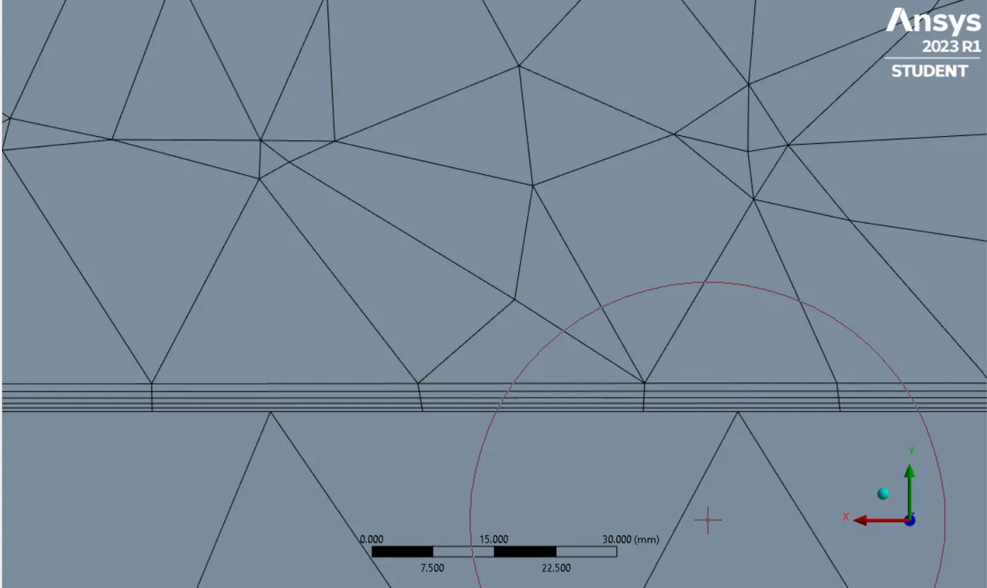
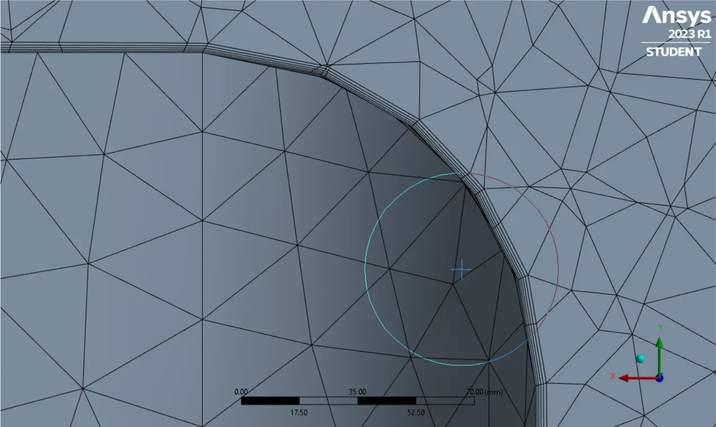
CASE - III:
Outer Enclosure - Multi Zone Method - 58mm
Inner Enclosure - Element size - 36mm
Inflation Layer - First Layer Thickness - 1.46mm
Method Selection:
From the research published by Thomas Hughes from the University of Derby under the title "CFD STUDY OF FLOW OVER A SIMPLIFIED CAR USING TURBULENCE MODELS", he carry out the research based upon the various slant angles 25degree, 35 degree and 45 degree and analyse which turbulence model will be the best suitable model for solving the simulation. On that he stated that K-Omega model and RSM (Reynold's Stress Model) would be more accurate than K-epsilon model, if the flow is linear( K-omega) may be used or if the flow complex (RSM) would be used or if it comprise both K-Epsilon is used.
And according to his research findings, RSM model will be accurate when the meshing refinement is good. And he also find out that for solving the slant angle lesser than 25 degree, K-Epsilon model gives the better result comparing to the other models as the error percentage of drag and lift is way better comparing to the K-omega and RSM model.
So for our studies as we are having the less computational power and also in our geometry the slant angle provided is 20 degree, we chose to solve our geometry in K-EPSILON MODEL.
Turbulence Model : K-Epsilon Model
Solver : Pressure Based Solver
Time : Steady
Method : SIMPLE (Semi-Implicit Method for Pressure Linked Equation)
Inlet Velocity : 25m/s
Temperature : 300K
Working Fluid : Air (with standard values)
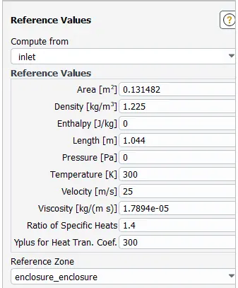
For calculation the drag and lift values, we have to properly provide the reference values to our simulation.
Y plus calculation:
PLOTS:
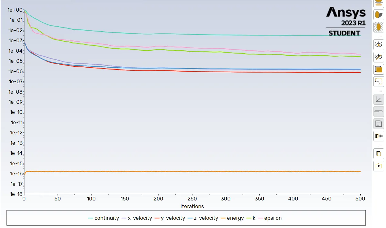
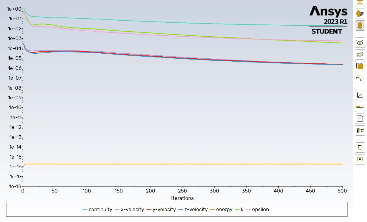
Residuals :
CASE -I CASE - II
(Automatic Meshing) (First Layer Thickness - 3mm)
CASE - III
(First Layer Thickness - 1.46mm)
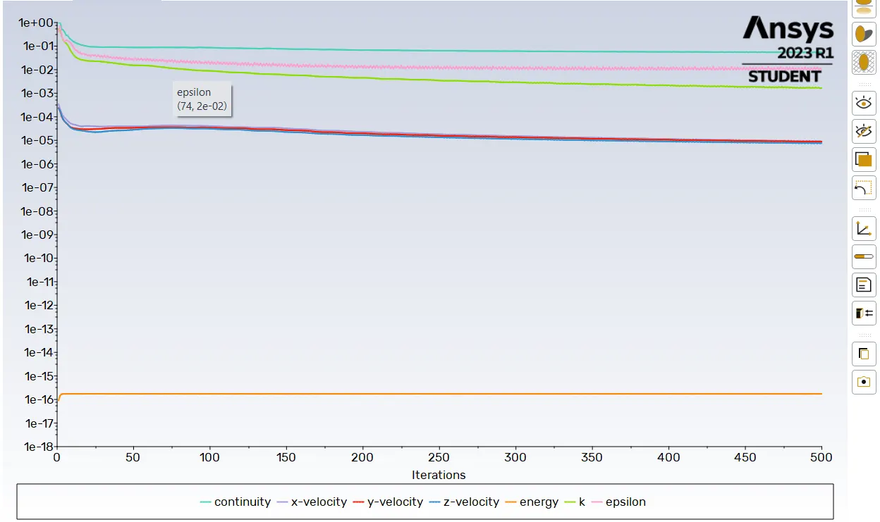
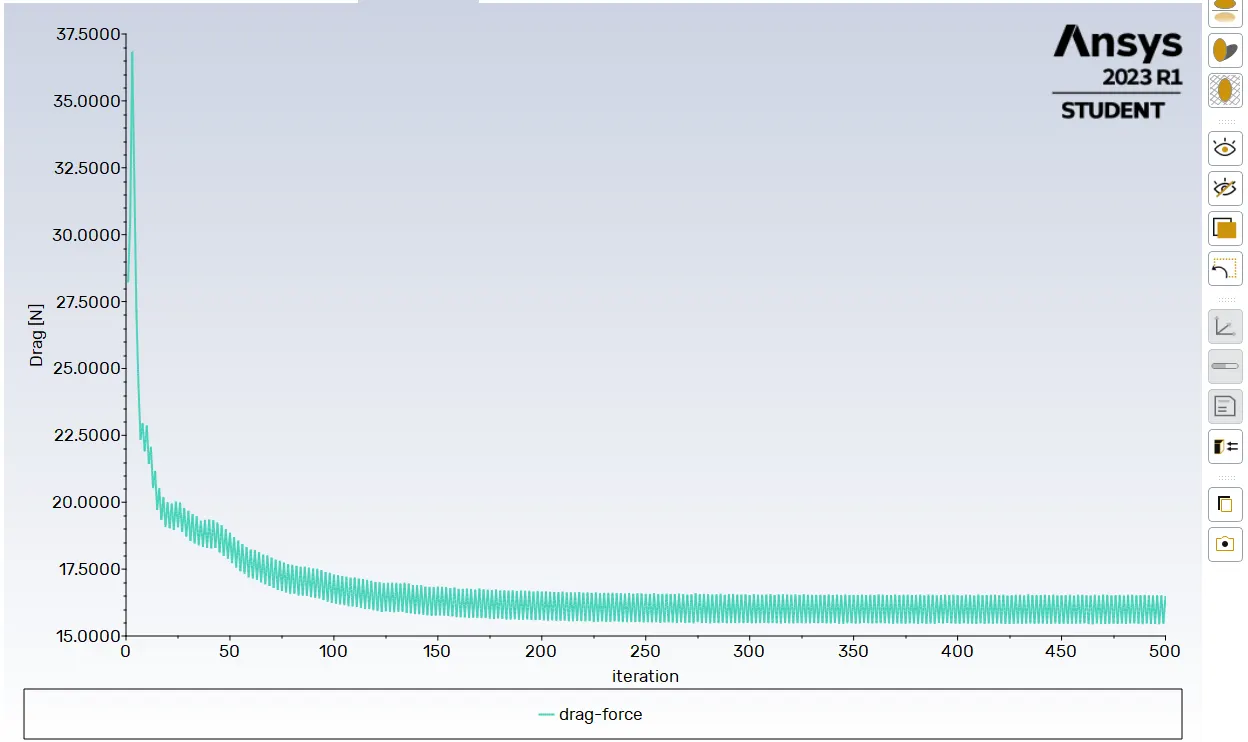
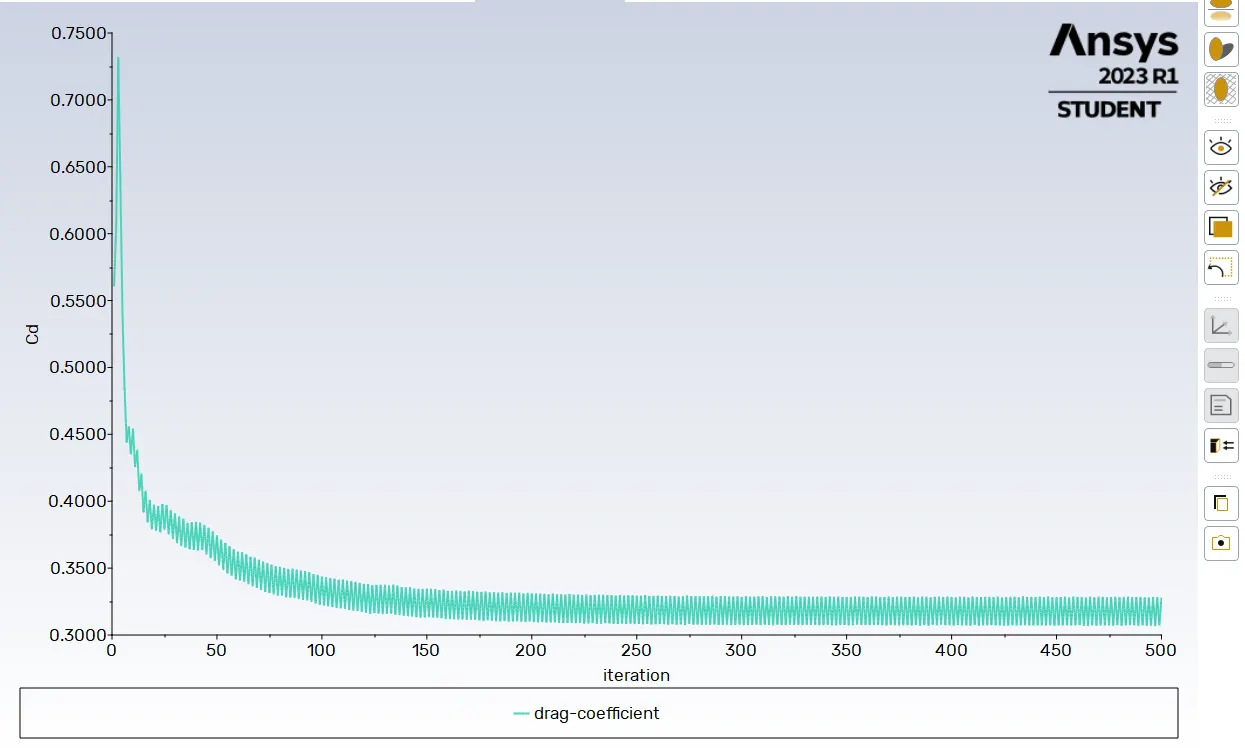
For checking the convergence in this simulation, we have to check the residuals as well as the drag coefficient, if the values are constant throughout the iteration then the solution is converged.
Drag Force :
From the observation results it is clearly seen that proper selection of the method for solving and the properly refined mesh will give us the better results.
CASE -I = 19.32N CASE - II = 16.54N
(Automatic Meshing) (First Layer Thickness - 3mm)
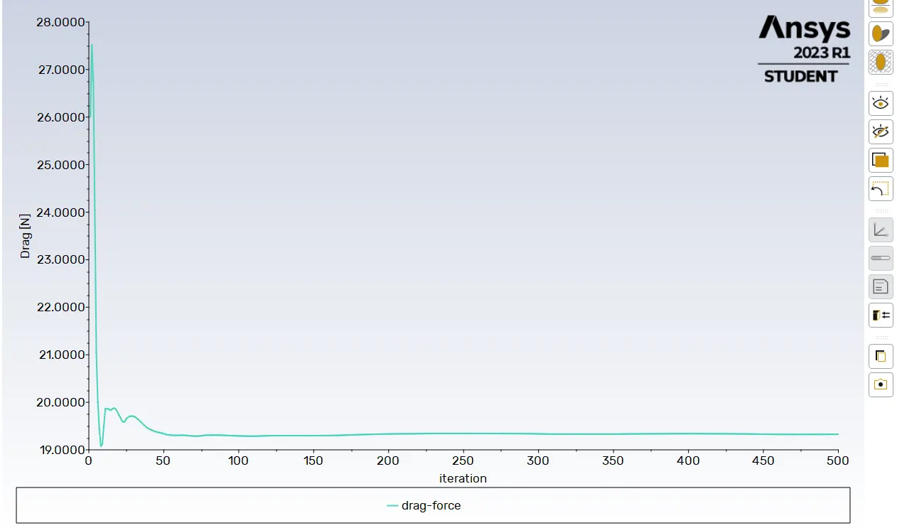
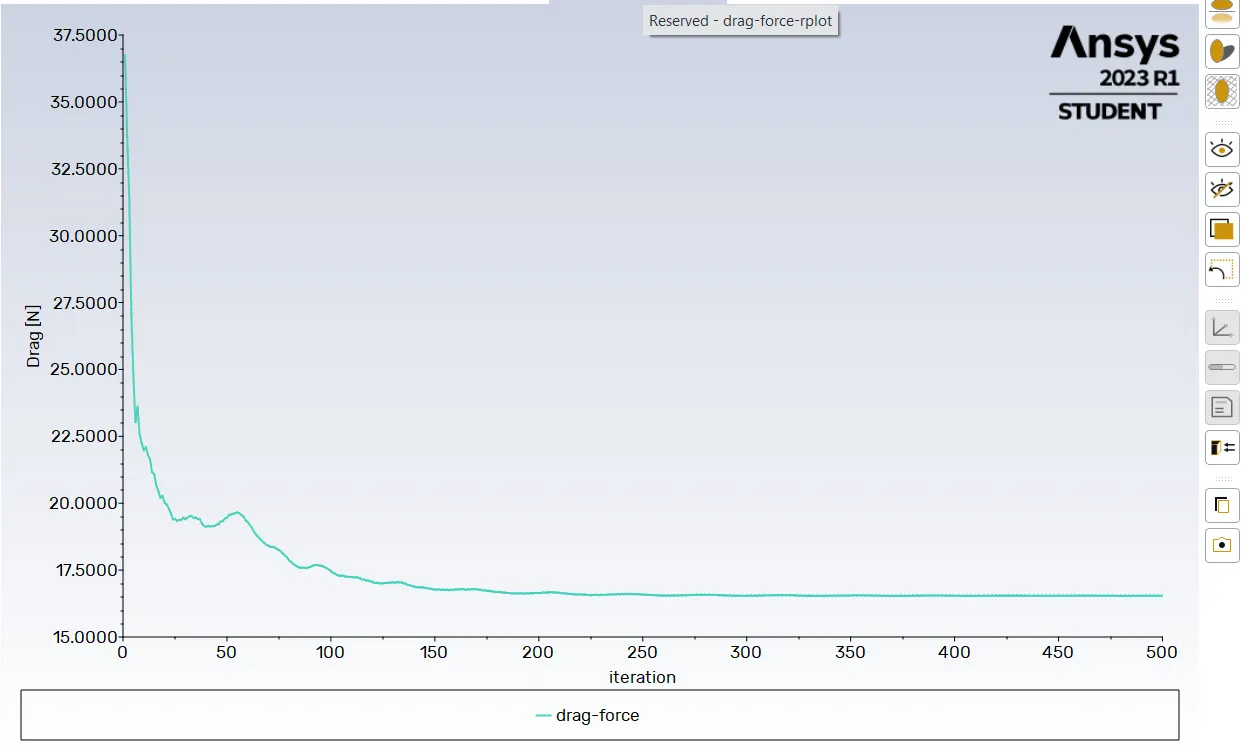
CASE - III = 16.48N
(First Layer Thickness - 1.46mm)
Drag Co-efficient:
CASE -I = 0.3839 CASE - II = 0.3275
(Automatic Meshing) (First Layer Thickness - 3mm)
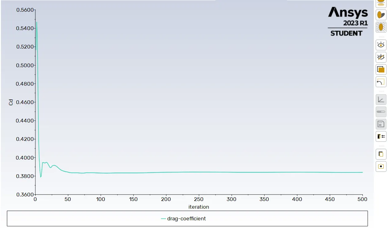
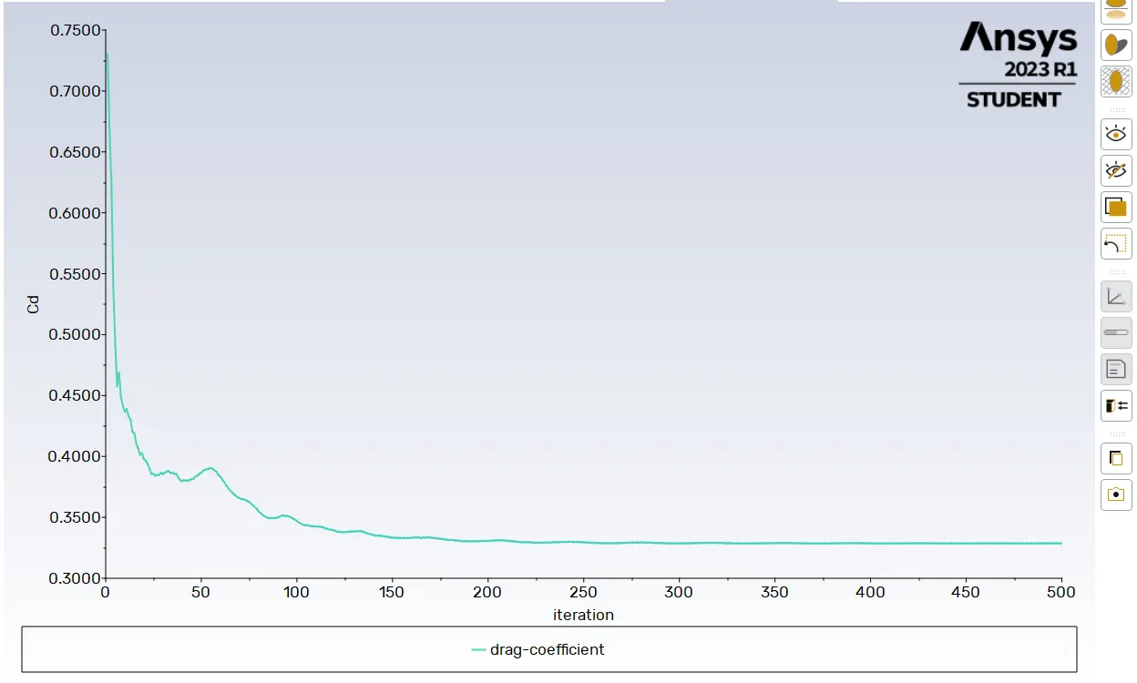
CASE - III = 0.3287
(First Layer Thickness - 1.46mm)
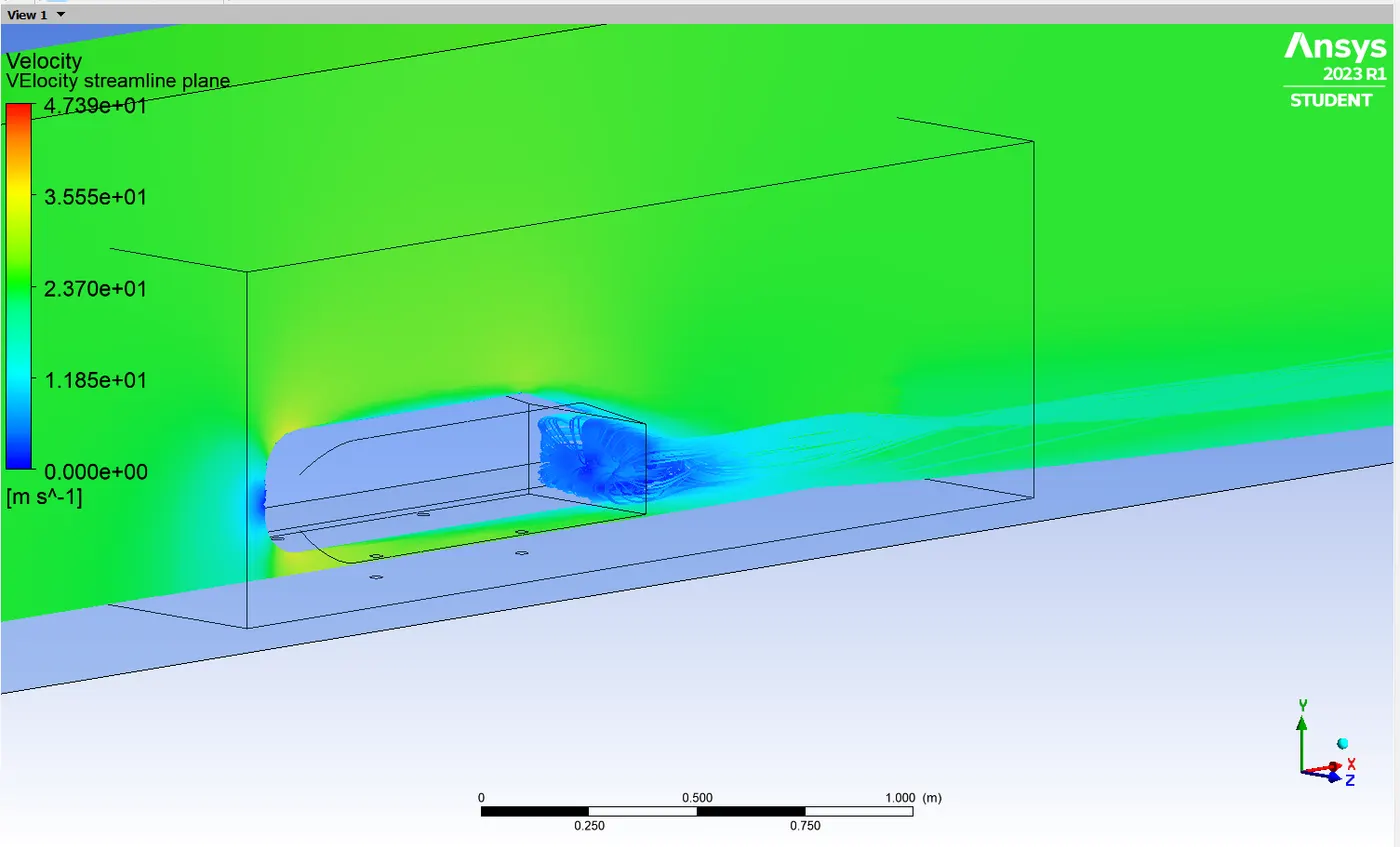
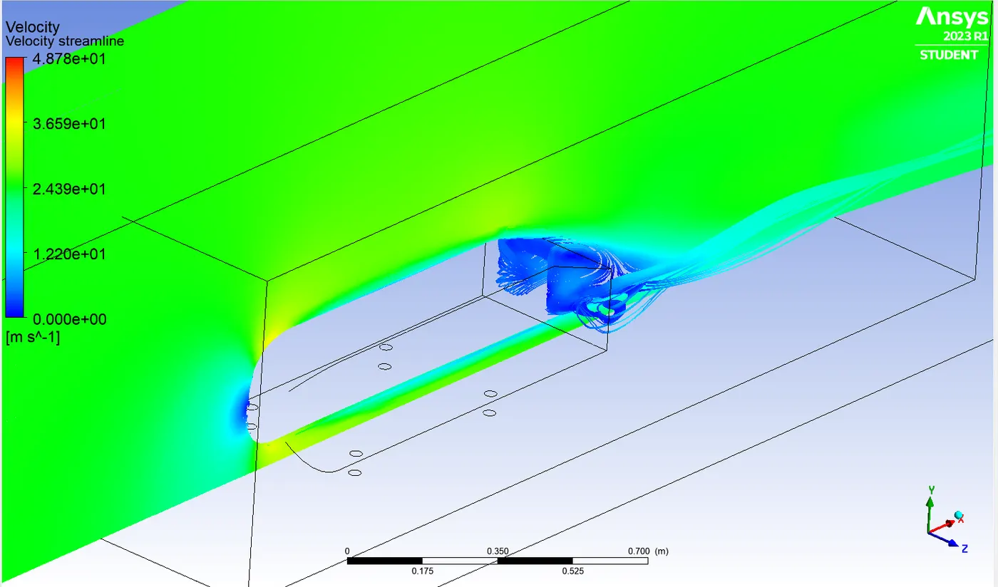
Velocity Streamlines:
CASE -I
(Automatic Meshing)
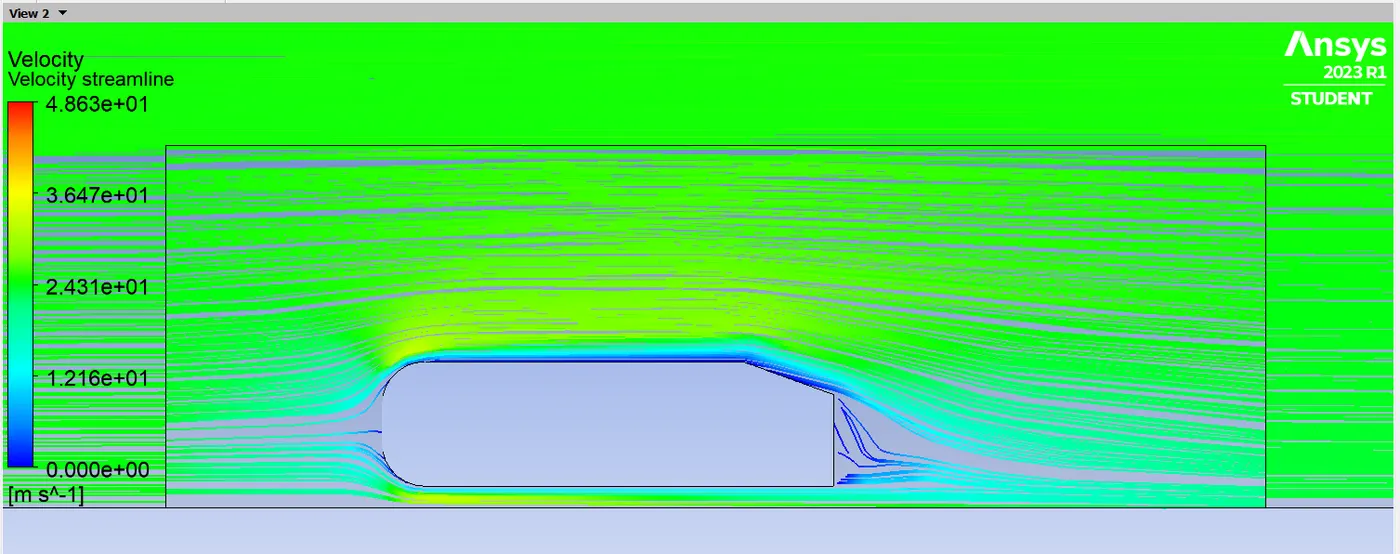
CASE - II CASE - III
(First Layer Thickness - 3mm) (First Layer Thickness - 1.46mm)
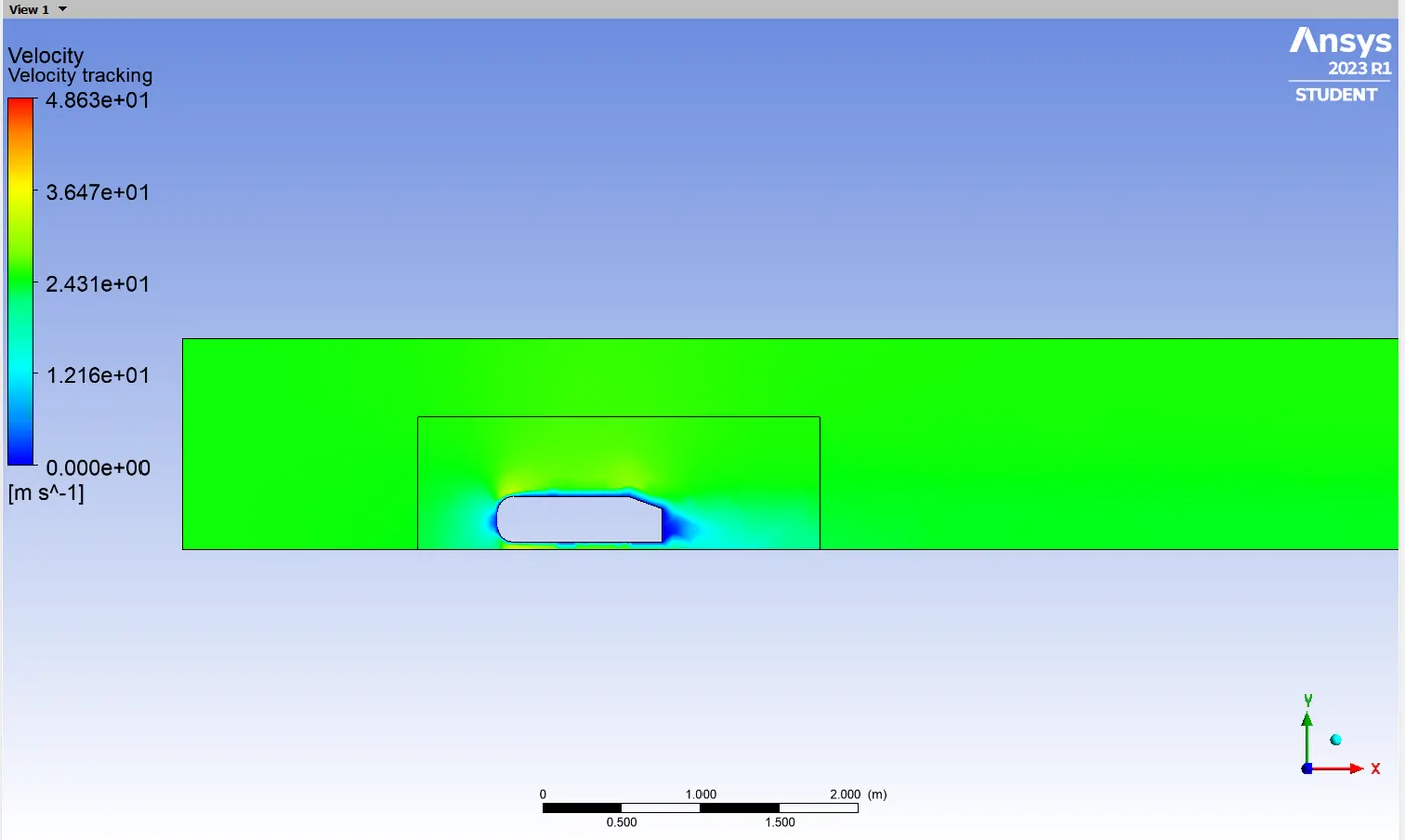
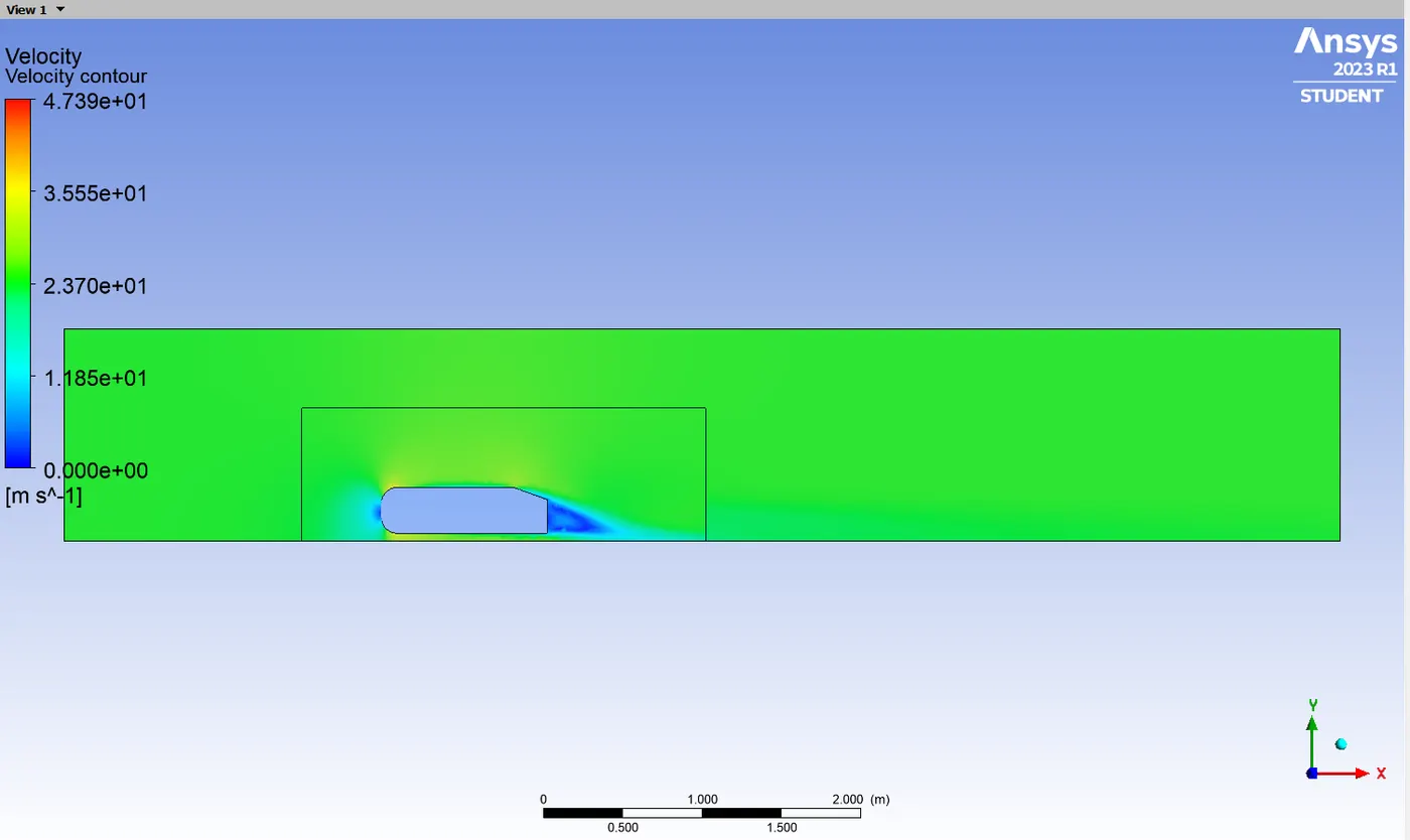
Velocity Distribution Contour:
CASE -I CASE - II
(Automatic Meshing) (First Layer Thickness - 3mm)
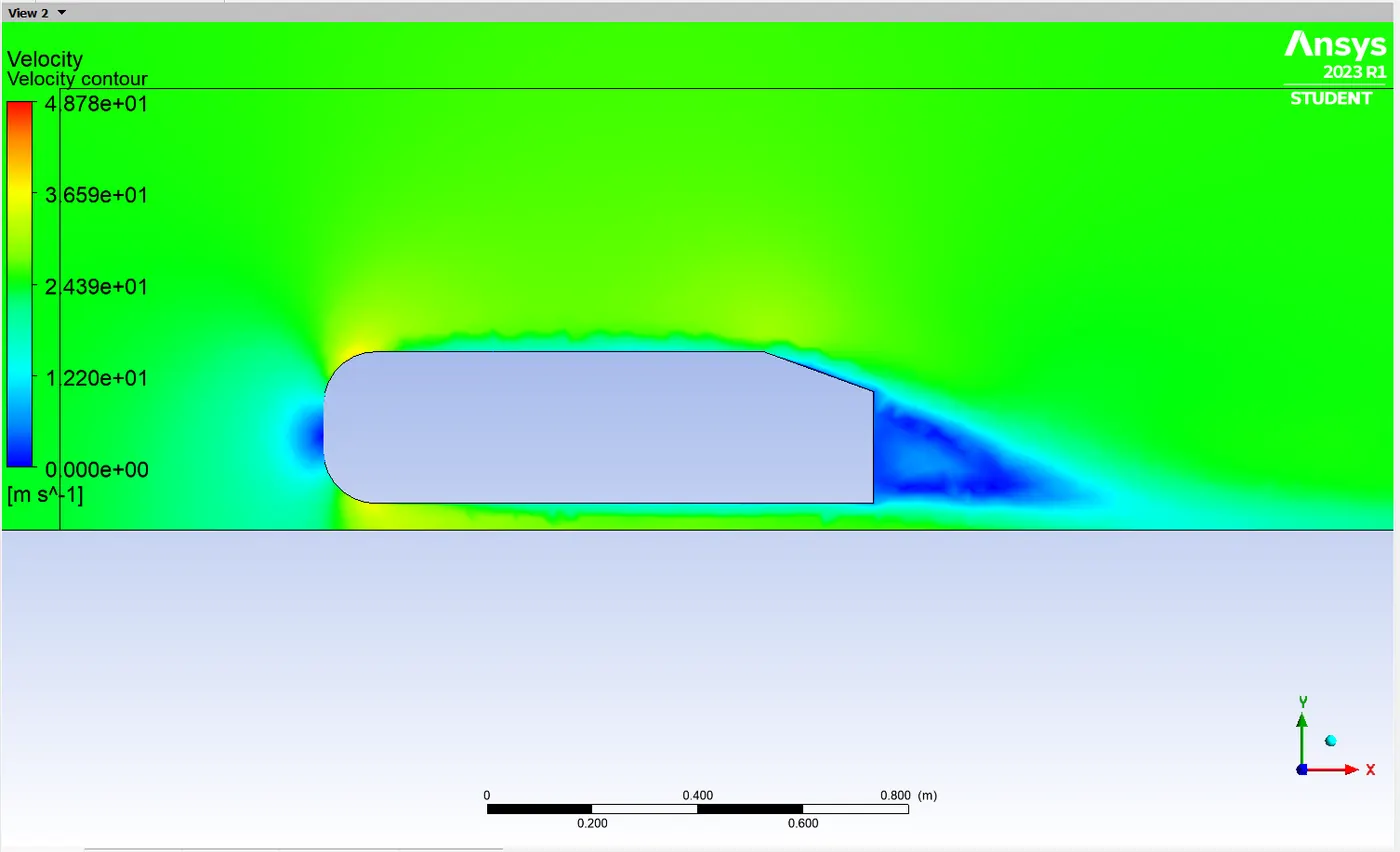
CASE - III
(First Layer Thickness - 1.46mm)
Velocity Distribution Plot:
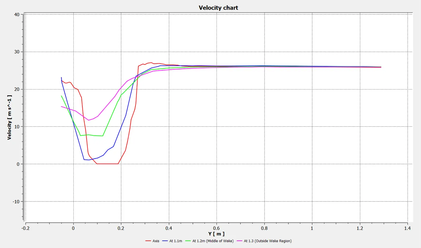
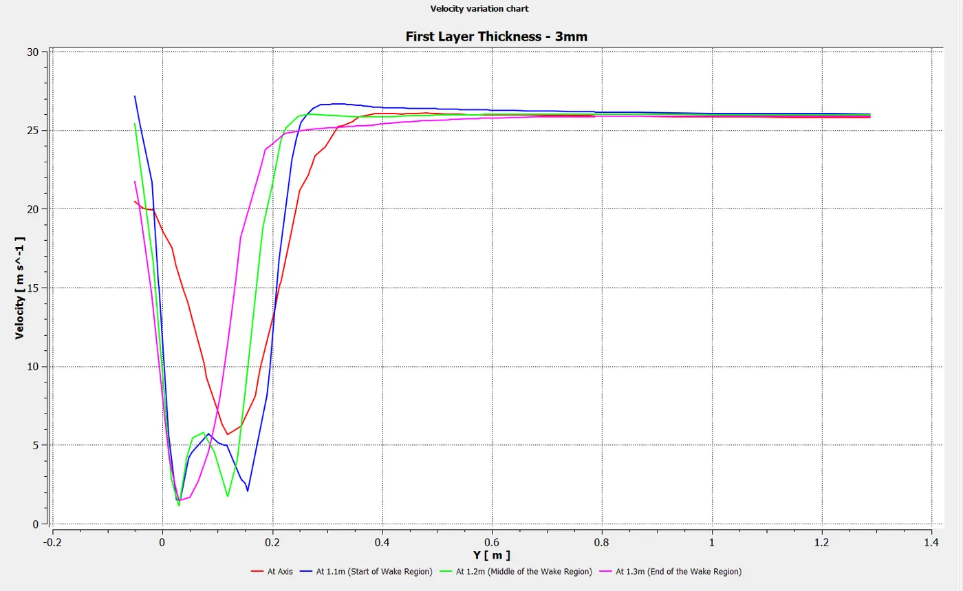
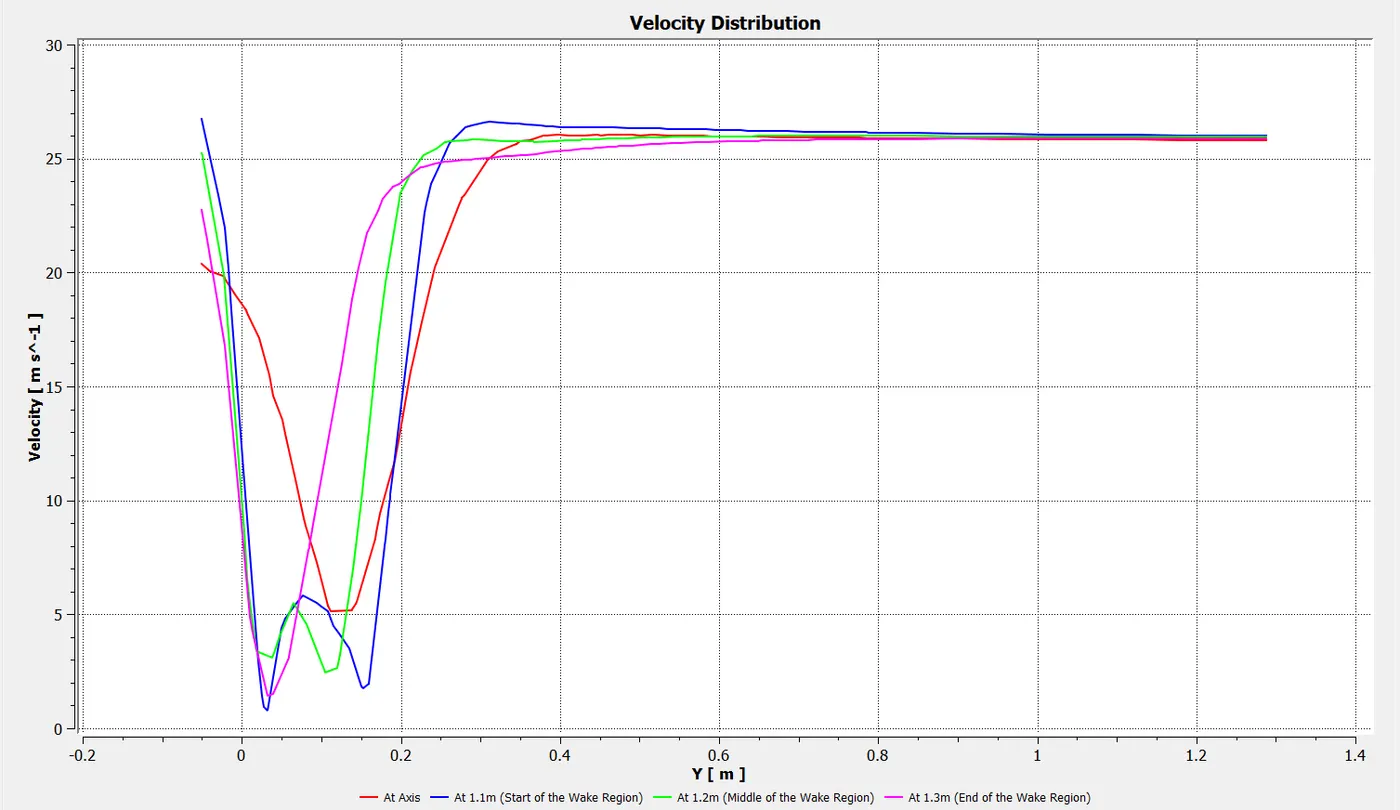
From the plot it is clearly noted that the velocity profile at the front end of the ahmed body and also at the wake region is very low compared to the outer surface of the body. The velocity reading noted at the axis (ahmed body front face), At 1.1m (Starting of the Wake region), At 1.2m(Middle of the wake region) and At 1.3m (End of the wake region).
CASE -I CASE - II
(Automatic Meshing) (First Layer Thickness - 3mm)
CASE - III
(First Layer Thickness - 1.46mm)
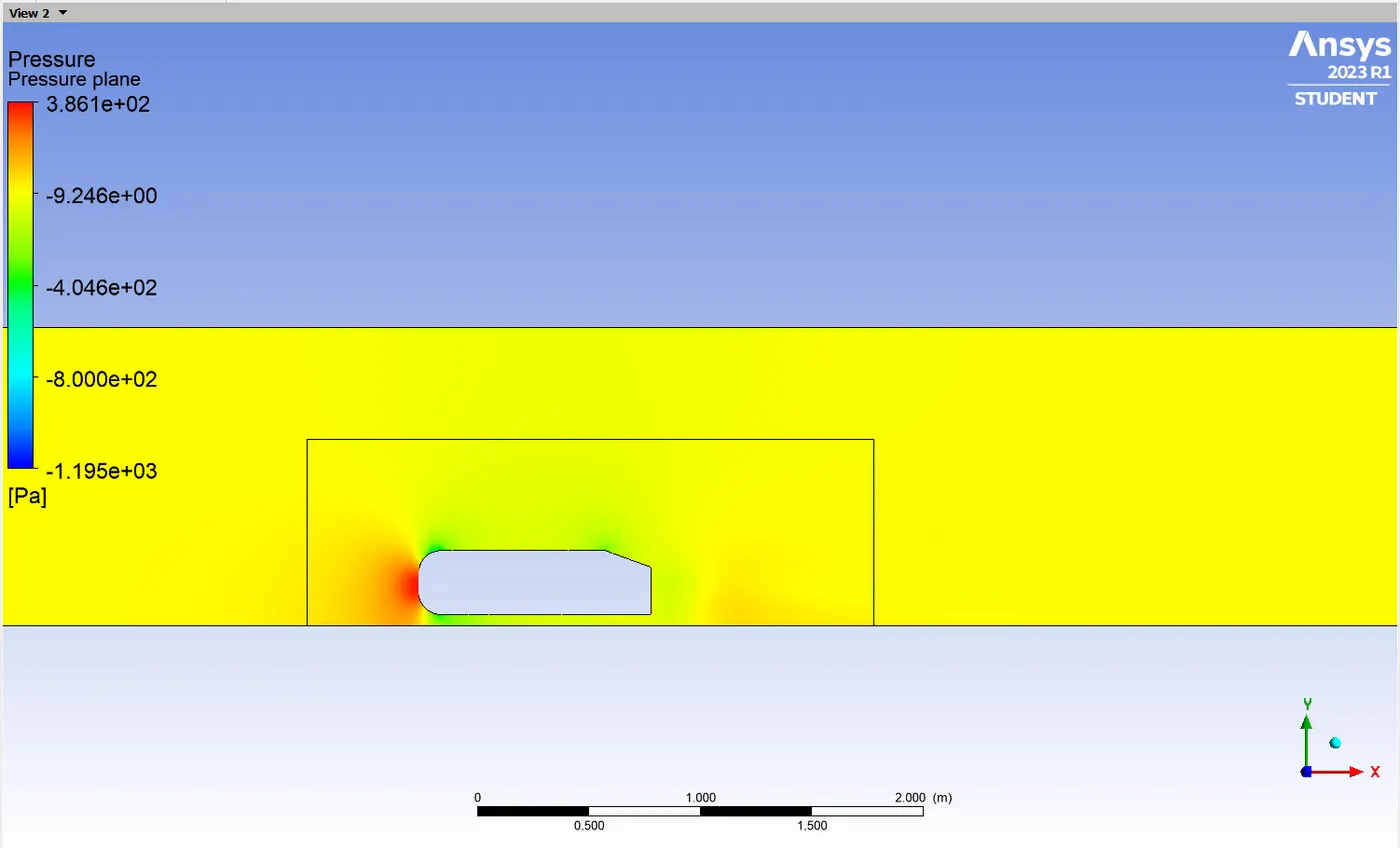
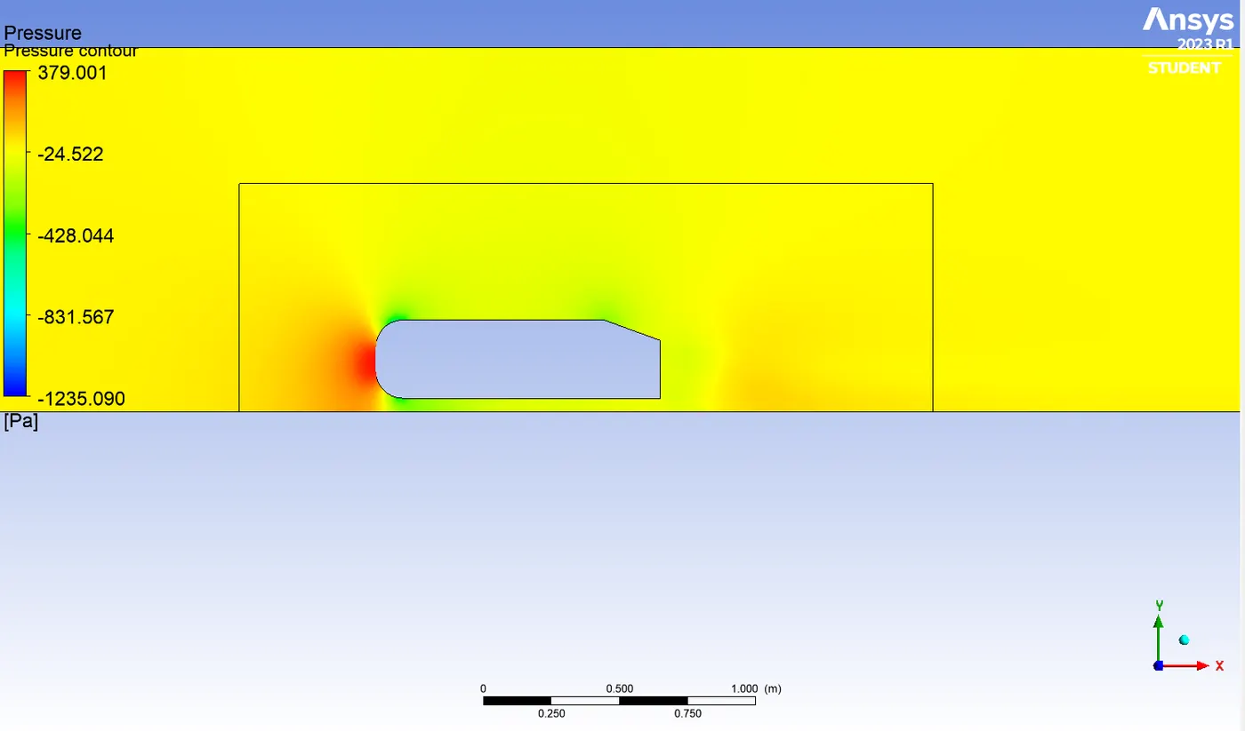
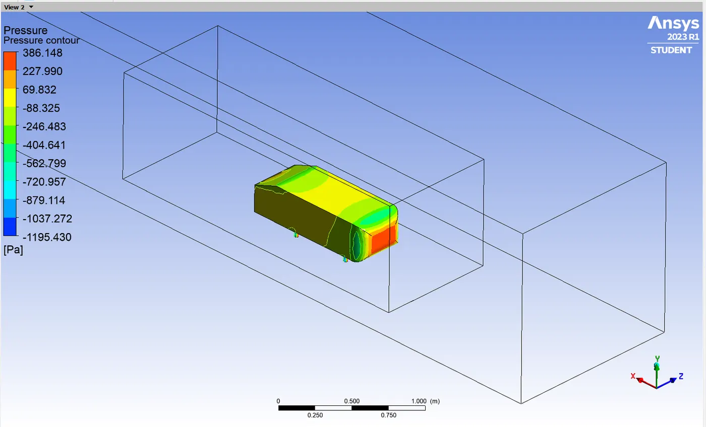
Pressure Distribution Contour:
CASE -I CASE - II
(Automatic Meshing) (First Layer Thickness - 3mm)
CASE - III
(First Layer Thickness - 1.46mm)
POINT OF SEPERATION (BOUNDARY LAYER SEPERATION):
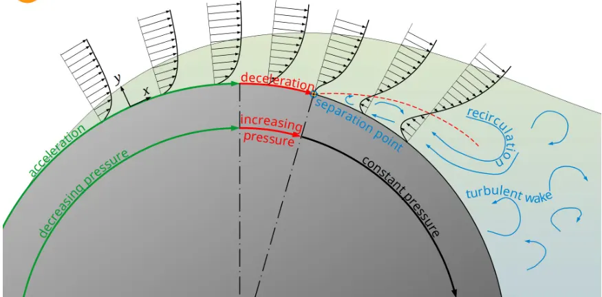
When a high reynolds number flow field is passed over a streamlined obstacle, relatively thin boundary layer forms on obstacle's surface. But whenever a high reynolds number flow field is passed over a non-streamlined obstacle, it leads stagnation point normal to the flow field in the obstacle causes thin boundary layer at that point. Relatively at the stagnation point the velocity is closer to zero, which can be seen in the velocity contour in our plot (The front face of the ahmed body has significantly very low velocity as it faces normal to the flow field). The thin boundary layer increases through the obstacle surface increases. After that the thin boundary layer seperates from the surface of the obstacle in the back and it will form a vortices behind it. This phenomenon is called as Boundary Layer Seperation.
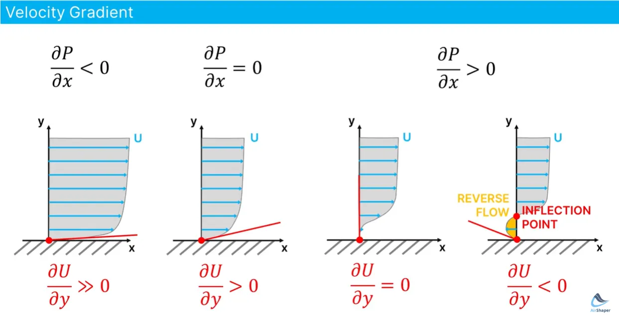
Boundary layer seperation is strongly associated with the adverse pressure gradient or strong flow deceleration
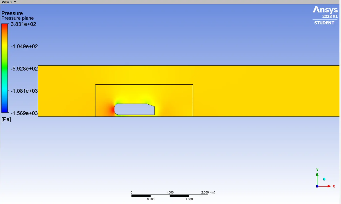
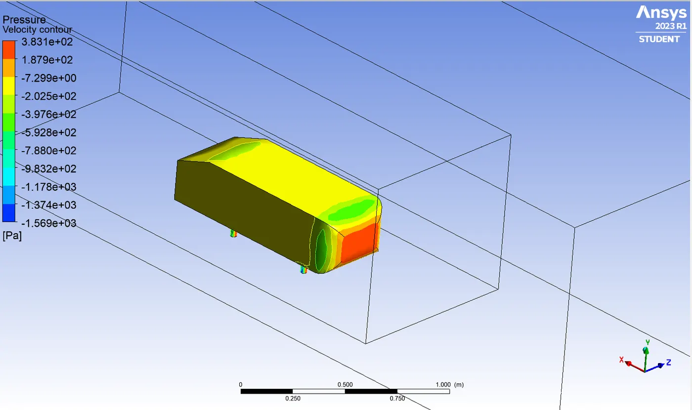
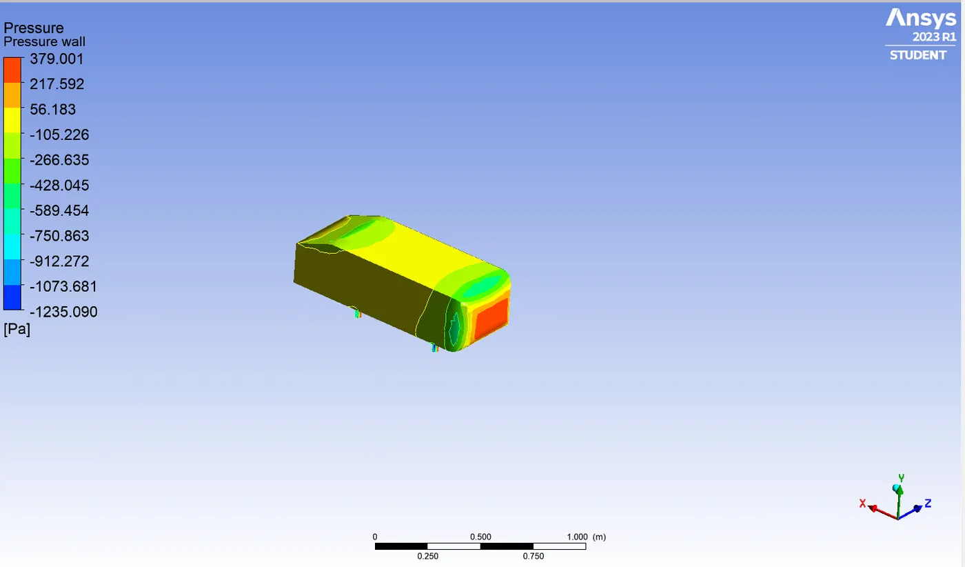
According to the Bernoullis principle, the pressure depends upon the undisturbed velocity flow. However the streamlined obstacle doesnot have the undisturbed velocity flow. But the non-streamlined obstacle such as Ahmed body have the disturbed velocity flow leads to the pressure gradient in the X direction. The flow over the ahmed body is upwards when flow faces the body and downwards when the flow leaves the body in order to flow around a ahmed body. But by the continuity equation of conservation of mass, same mass to be maintained in the system inorder to that increase in flow velocity happens at this point. It is clearly seen in our Velocity contour plot, that after the flow faced by the ahmed body there is a low velocity occurs but at the edge of the front face there is a increase in velocity. This happened due to the conservation of mass. So as stated in bernoullis equation, increase in velocity decrease will be the pressure and vice versa. This can be seen while comparing the velocity contour and pressure contour plot we had during simulation. After certain point the pressure get increased and obstruct the flow field which inturn called as adverse pressure gradient.
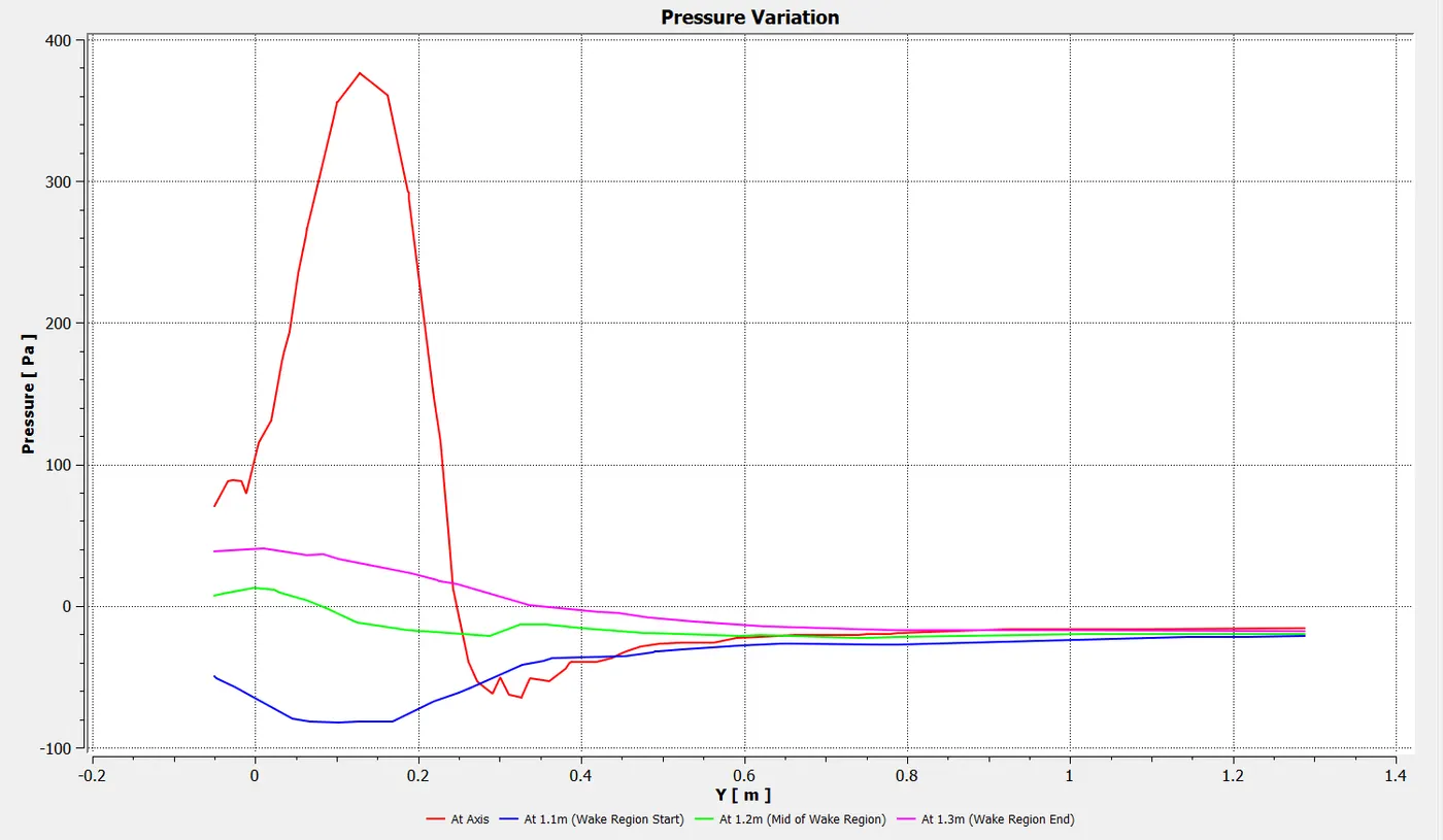
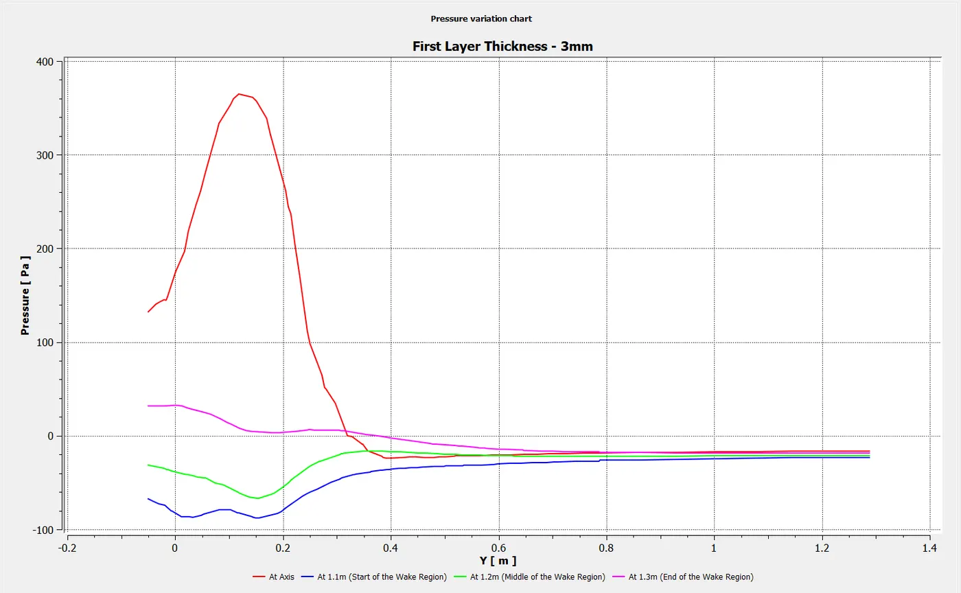
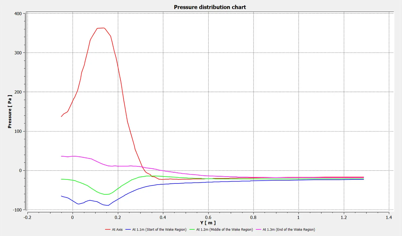
Pressure Distribution Plot:
CASE -I CASE - II
(Automatic Meshing) (First Layer Thickness - 3mm)
CASE - III
(First Layer Thickness - 1.46mm)
Pressure Distribution At Car Wall:
CASE -I CASE - II
(Automatic Meshing) (First Layer Thickness - 3mm)
CASE - III
(First Layer Thickness - 1.46mm)
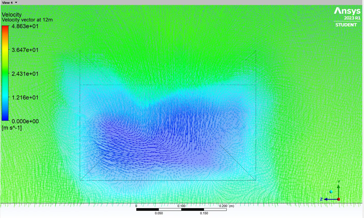
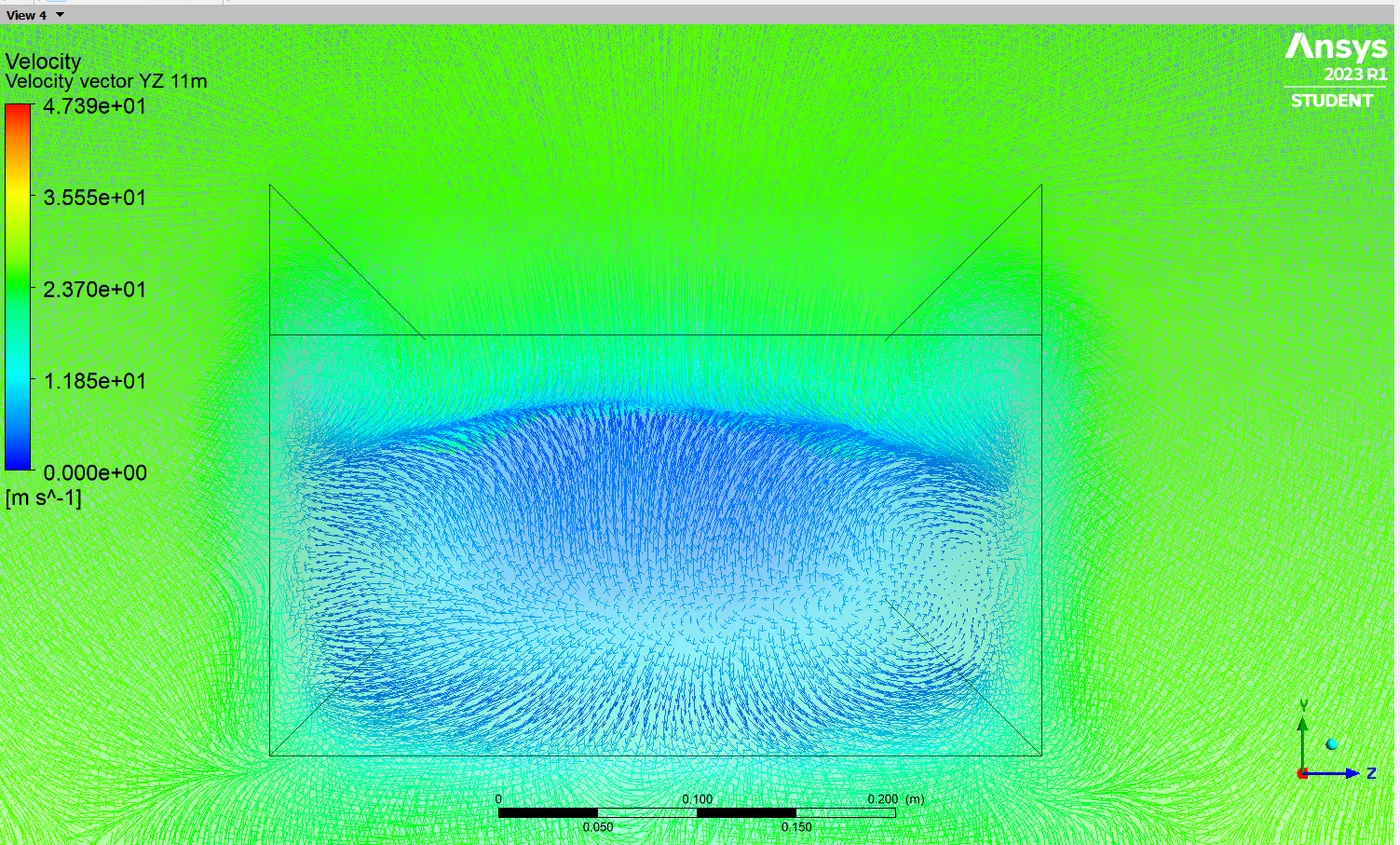
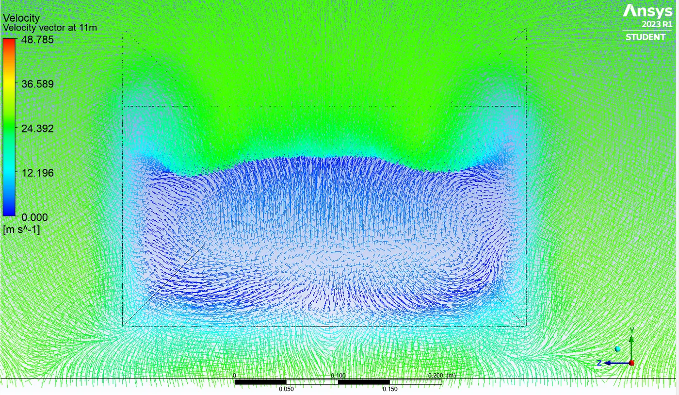
Velocity Vector Plot (At the Starting of the Wake Region):
CASE -I (At 1.1m) CASE - II (At 1.1m)
(Automatic Meshing) (First Layer Thickness - 3mm)
CASE - III (At 1.1m)
(First Layer Thickness - 1.46mm)
Reason for Negative Pressure in the wake Region:
As we seen it in the Pressure distribution chart one of the results obtained in our simulation. At the start, middle and end of the wake region low pressure(Negative pressure) is observed. From the observation the negative pressure is high near to the rear side of the ahmed body and the pressure is increased over the flow. By the end of the wake region the pressure touches the nominal pressure range. This is the observation from our study.
At the initial condition with out the flow happens, the particles at the rear side of the ahmed body stays constant. When the flow happens around the ahmed body, after the seperation occured at the slant angle provided at the rear, the particles are moving at the faster rate due to the flow. This high speed moving particle intacts with the particles at constant behind the ahmed body and creates the shear stress plane. The velocity above the shear stress plane is very high comparing to the below. This shear stress causes the flow to get rotational and formation of the vortices happens. This generally occurs at the high reynolds number, where the shear stress is also high. The generated vortices are having the lower pressure at its own axis. This will leads to the lower pressure at the wake region. This low pressure (negative pressure) will vary with the speed of the flow, characteristics of the flow and also by the shape of the body.
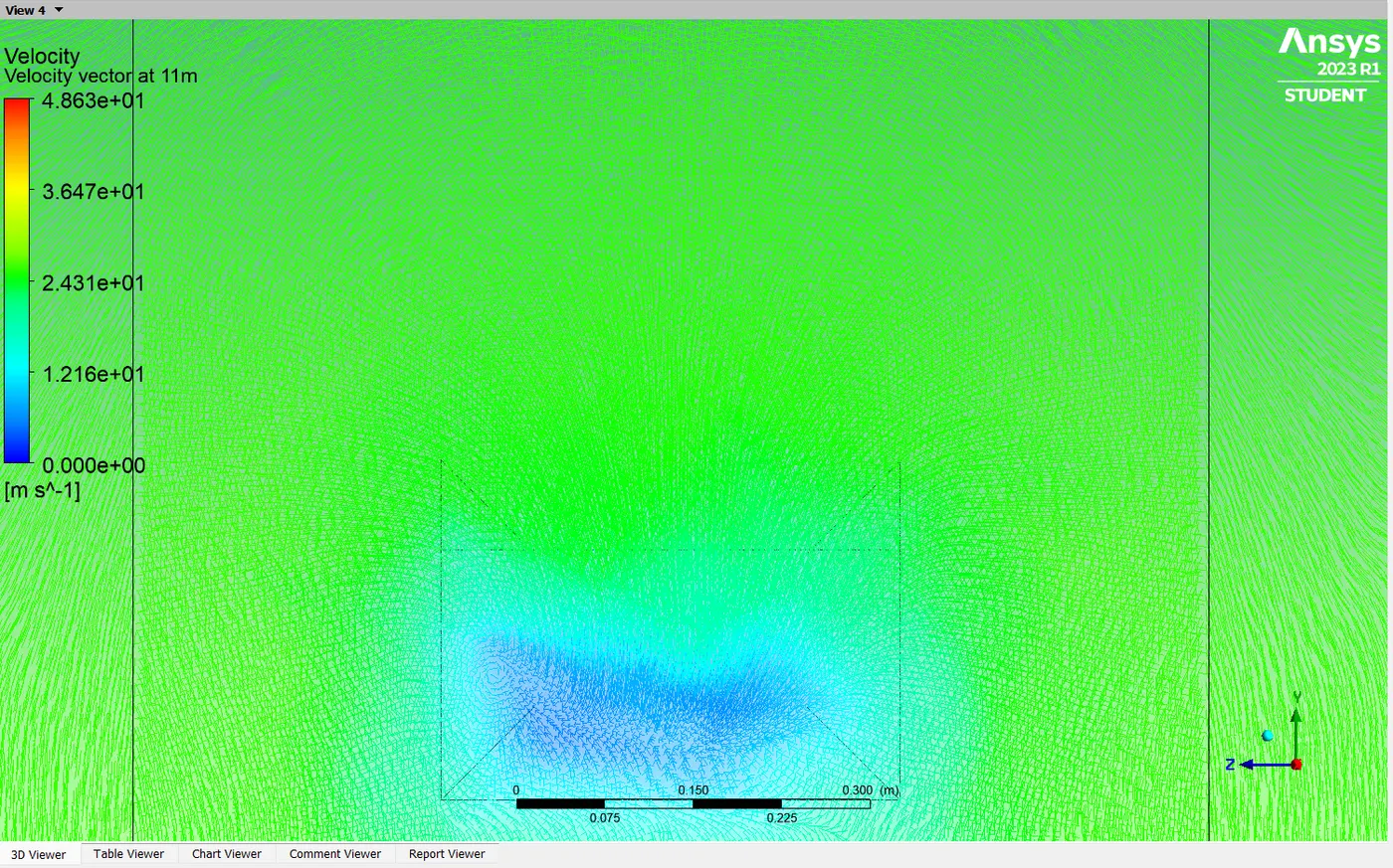
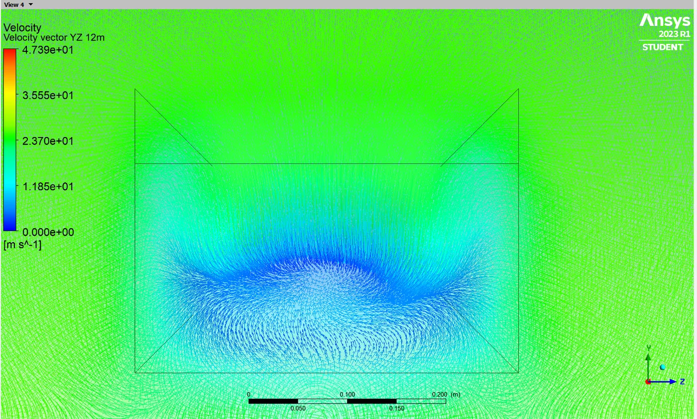
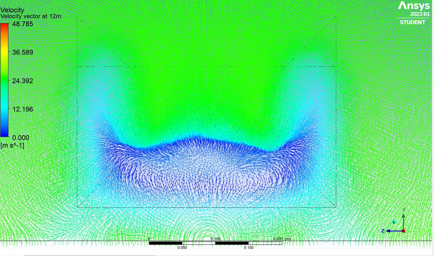
From the velocity vector plot it is clearly seen that the vortices are generated at the two ends along the Z axis.
Velocity Vector Plot (At the Middle of the Wake Region):
CASE -I (At 1.2m) CASE - II (At 1.2m)
(Automatic Meshing) (First Layer Thickness - 3mm)
CASE - III (At 1.2m)
(First Layer Thickness - 1.46mm)
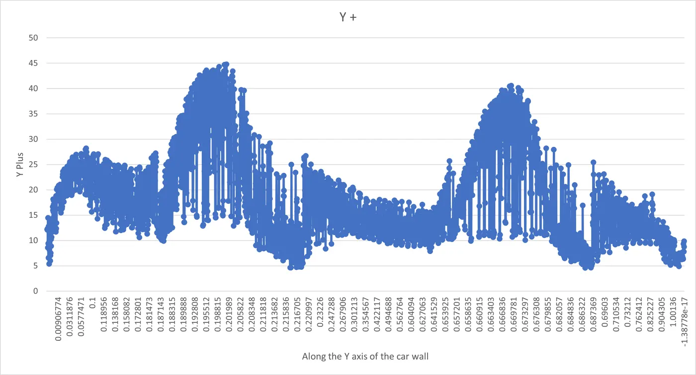
Y - Plus :
CASE - I = 537.7114 CASE - II = 31.8604
(Automatic Meshing) (First Layer Thickness - 3mm)
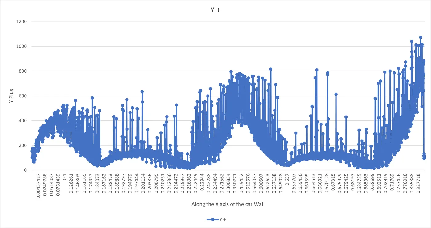
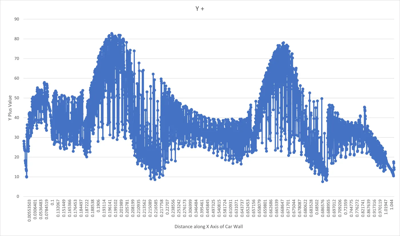
CASE - III = 13.7762
(First Layer Thickness - 1.46mm)
Mesh Indepedence Study:
| Cases | Method | Element Count | Drag Coefficient | Drag Force (N) | Obtained Y-Plus | Error % of Drag Coefficient |
| I | K-Epsilon | 80929 | 0.3839 | 19.32 | 537.7114 | 14% |
| II | K-Epsilon | 351170 | 0.3275 | 16.54 | 31.8604 | 0.75% |
| III | K-Epsilon | 477694 | 0.3287 | 16.48 | 13.7762 | 0.39% |
RESULTS:
Thus the flow over a Ahmed body with slant angle of 20 degree at velocity 25m/s is simulated and also understand about the flow behaviour over the ahmed body. The concepts of point of seperation, wake and the vortices are also clearly understood as we can visually seen it from our resultant plots and images at the end of the simulation. The mesh independence study also conducted and got the clear view of how the meshing will increase the efficiency of the results.
LEARNING OUTCOMES:
- Clear understanding of Ahmed Body
- Understood the concept of Boundary Layer theory
- Significance of point of seperation in boundary layer theory
- Negative pressure in the wake region and its causes
- Mesh independence study.
- Calculation of Y plus values and its significance.
REFERENCES:
- Some salient features of the time-averaged ground vehicle wake by S.R. Ahmed and G.Ramm
- CFD study of flow over a simplified car(Ahmed body) using different turbulence models by thomas Hughes, University of Derby
- Flow and turbulent structures in the wake of a simplified car (Ahmed body) by S.Becker, University of Erlangen