Week 3 - External flow simulation over an Ahmed body.

Week 3 - External Flow simulation over an Ahmed Body.

Aim:

To Simulate the external flow over an Ahmed Body, perform grid in-dependency test and study for drag and lift values in each case.

We shall study for 3 case

Case	Outer enclosure element size (mm)	Inner enclosure element size (mm)	Car wall element size (mm)
Case 1	250	100	5
Case 2	100	50	3
Case 3	80	45	3

Introduction:

Ahmed Body and its importance:

The Ahmed body is a benchmark model widely used in the automotive industry for validating simulation tools. The Ahmed body shape is simple enough to model, while maintaining car-like geometry features

The Ahmed Body was first created by S.R. Ahmed in his research “Some Salient Features of the Time-Averaged Ground Vehicle Wake” in 1984. Since then, it has become a benchmark for aerodynamic simulation tools. The simple geometrical shape has a length of 1.044 meters, height of 0.288 meters, and a width of 0.389 meters. It also has 0.5-meter cylindrical legs attached to the bottom of the body and the rear surface has a slant that falls off at 40 degrees.

Negative pressure in the wake region:

As the air flows over the Ahmed Body, the flow separation starts at the slant face interface. Although there is a possibility of mixing of air at this zone at lower speeds, at higher velocities the velocity of the moving fluid contributes to the wake region. This not only creates a wake region, but retains it along the flow.

The air becomes almost stagnant as it strikes the vehicle which results in air exerting very high pressure on front of the vehicle. The airflow then gets divided between the upper and lower surface of the vehicle. The higher pressure air on front surface accelerates as it travels over the curved nose surface of Ahmed body, causing the pressure to drop. This lower pressure creates lifts over the roof surface as the air passes over it. As the air continues to flow and make its way to the rear, a notch is created by the rear slant owing to flow separation, leaving a vacuum or low pressure space which the air is not able to fill properly. The resulting lower pressure creates lift that then acts upon the surface area of the rear slant. This is the reason for the negative pressure in the wake region.

Point of Separation:

The point of separation is the point where the flow starts to separate on the Ahmed Body, this is the interface of the roof and the slant rear face. The point of separation and the angle of the slant face contributes to the pressure of the wake region and the aerodynamics of the Ahmed body. This angle is called ‘Alpha’ angle. There are some open literature studying the impact of angle on the pressure of the Ahmed Body.

Solving and Modeling approach:

We shall solve for 3 cases as discussed in Aim.We will be using ANSYS Fluent solver to create the geometry and perform unstructured tetra CFD mesh with boundary definitions, setup the physics of fluid flow and run the iterations to get solutions, using post processing to interpret the data in form of plots,contours, vectors, streamlines etc.,

With velocity of 25 m/s and k-epsilon model we shall study grid independence for Ahmed Body with RANS. When we say grid independence study we shall study for 3 cases as follows.

Case	Outer enclosure element size (mm)	Inner enclosure element size (mm)	Car wall element size (mm)
Case 1	250	100	5
Case 2	100	50	3
Case 3	80	45	3

We shall keep in mind we are using a student version of ASNYS, so we are limited with the number of elements to play with. Then, we tabulate the case study results and compare it with the open literature or book data results to validate the simulation.

Preprocessing and Solver setting:

Let us open ANSYS workbench, now opening Fluent flow can be done by drag and drop in the schematic window or by double clicking on Fluent. The fluent workflow is in a series of steps such as GEOMETRY > MESH > SETUP > SOLUTION > RESULTS. Each step has to be completed for the next step to initialize.

In the grid independence study we shall consider case 2 and discuss in detail,

GEOMETRY >

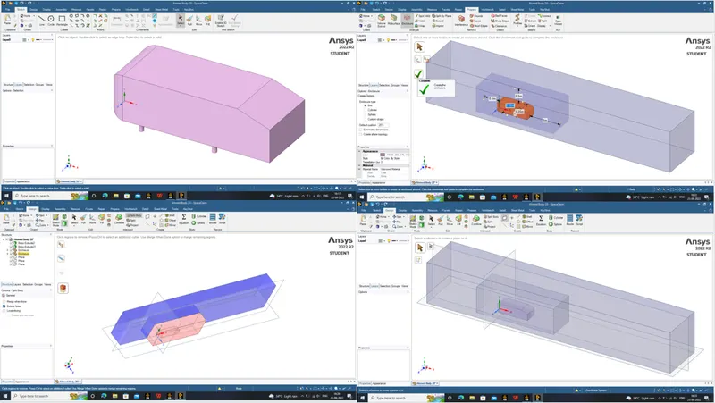
In the Fluent, right click on the Geometry and select New SpaceClaim Geometry. The space claim application opens, select FILE > OPEN and open the Ahmed Body model.

For flow study we need Flow domain, we shall create one using ENCLOSURE option. Since we are limited with the number of elements and we need more accuracy only near to the car, we can create an inner enclosure near to the car using the same ENCLOSURE option, un-checking the symmetry we should be able to define distances at all direction. The enclosure dimensions are as follows;

	Front (m)	Back (m)	Top (m)	Bottom (m)	Side (m)
Outer enclosure	2	5	1	0	0.5
Inner enclosure	0.5	1	0.5	0	0.25

Since the Ahmed Body is a perfectly symmetric body, we can create PLANE at the centre and use SPLITBODY command to delete the half of the model.

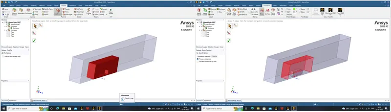
There are two enclosures, so we need to perform some more operations so that they behave as a single flow domain during study. INTERFERENCE option automatically identifies interference in objects and rectifies them, SHARE TOPOLOGY option shares the faces between 2 fluid volumes in this case the interface of outer and inner enclosures.

We are good to go now. Once the geometry is ready, we can close space claim and check that the fluid flow (fluent) geometry is updated indicated by a green tick.

MESH >

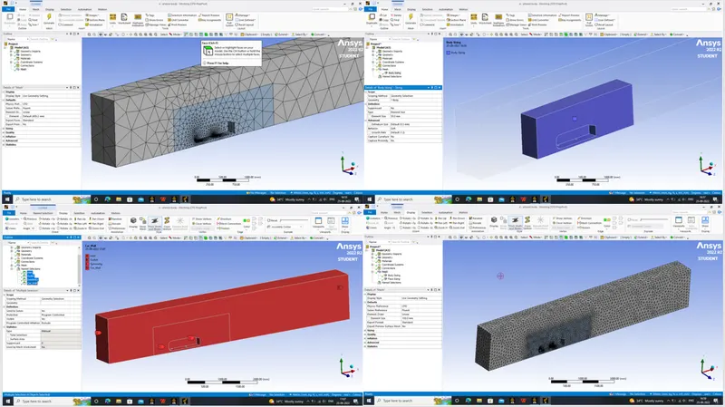
Right clicking on the Mesh and selecting edit opens the Mesh window. Mesh window is preloaded with the geometry we have worked on earlier, so clicking on the GENERATE MESH should create a mesh automatically.

For case 2 we are interested in a certain mesh size, that can be obtained by selecting the faces of car wall using FACE select option. And selecting the inner enclosure by BODY select option and in MESH > INSERT > SIZING we should be able to select and input desired mesh sizes for car wall and inner enclosure. For outer enclosure, we can input size at the mesh details itself.

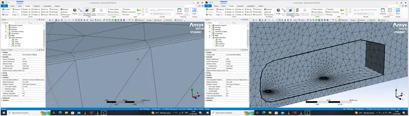
We shall use INFLATION layers for the car wall with 0.5 as first layer thickness with 6 layers and 1.2 as growth factor. Since we already used share topology option, the mesh should look good.

. Any changes made, click on the update icon to update the mesh details or else there is an indication of a thunderbolt sign asking the user to update.

We shall name the entry and exit surfaces such as Inlet, Outlet, Wall by selecting the respective faces and using the ‘N’ button and name them as symmetry. We shall select the car wall and name it as car wall. Once this is done, we should see a green tick near Mesh. we can close the mesh window.

SETUP >

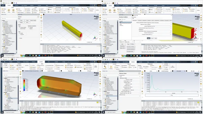
Right clicking on the Setup, opens the Fluent launcher. In the Fluent launcher select 3D, Double precision and select the number of cores as per the user system configuration and click on start.

Upon opening, there are some selections to be done to define the simulation definitions, we shall select Type: Pressure based, Velocity Formulation: Absolute, Time: Steady. Under the Physics tab, we can turn on viscous and select k-epsilon > Enhanced wall treatment as well.

Under the materials we shall select air as our default material with material type as fluid.

Under the cell zone conditions, select the volume and it should show type as fluid by default.

We can proceed to define boundary conditions, as follows

Inlet X : velocity magnitude = 25 m/s

Outlet should be a pressure outlet.

For generating surface reports, click on the Solution > Reports > Definitions > New > Force Report > Drag coefficient for the drag coefficient over the cylinder wall. Similarly we can make a report for lift coefficient.

We shall input compute from INLET in reference values and in the initialization as well. Now, it's time to start the simulation. In order to start the simulation for the above set up physics, we need to initialize the entire flow field by clicking on the t=0 initialize icon. In the Run Calculation we can input the number of iterations to be run (in this case 500) and clicking on the Calculate should start the iterations. After iterations, we get scaled residuals, average temperature plot and standard deviation plots.

We need velocity and pressure contours as well, to get them we can create a transverse cut plane i.e, XY plane and make new contour in Results > Graphics > Contours > New pressure for pressure contour and velocity for velocity contour. The scale can be edited by double clicking on it.

In the Outline view under Simulation Reports, clicking on the Report Outline > Generate should generate a Ansys Fluent Simulation Report which is automatically generated with all the information of the simulation in it. This can be exported as a PDF also. We are done with setup, we can close the setup.

SOLUTION >

Since some solution is calculated in the setup itself, we can see the green ticks in both setup and solution too.

RESULTS >

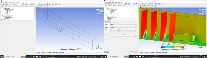
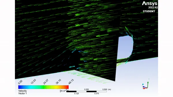
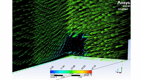
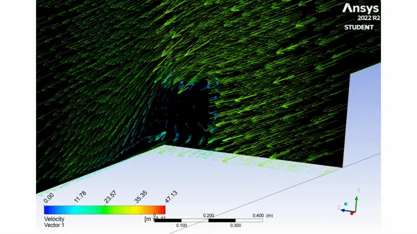
Right clicking on the Results should open the Post processor. Default view is a wireframe model, we can create a plane in XY to view contours and vectors. Selecting the Vector and selecting the plane creates a velocity vector.

Similar to setup and solution, all contours and plots can be created here, in addition to that we can create an animation of the velocity contour by clicking on AUTOSAVE during the solution and clicking on ANIMATE select make movie and save in desired location.

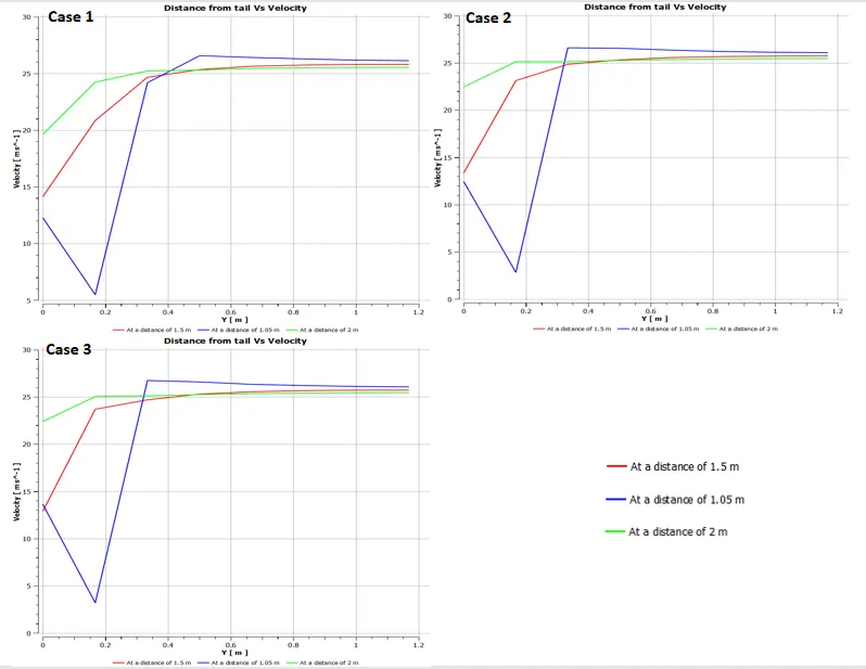
We shall create lines at distance of 1.05 m, 1.5 m, 2 m away from the tail of the car to study the velocity plots on the same. Plots can be created using the CHART option.

For Case 1 and Case 3, we shall repeat the same except for changing the grid size in meshing step. We can simply DUPLICATE case 2 fluent file and edit in it.

RESULTS:

After repeating the similar manner of simulation procedures for all 3 cases from aim, we have a handful of data to compare and study. We shall put in order all the contours, plots and vectors for us to compare and come to a conclusion. Here, only the results of all cases are displayed, its inference and interpretation shall be discussed briefly in conclusion.

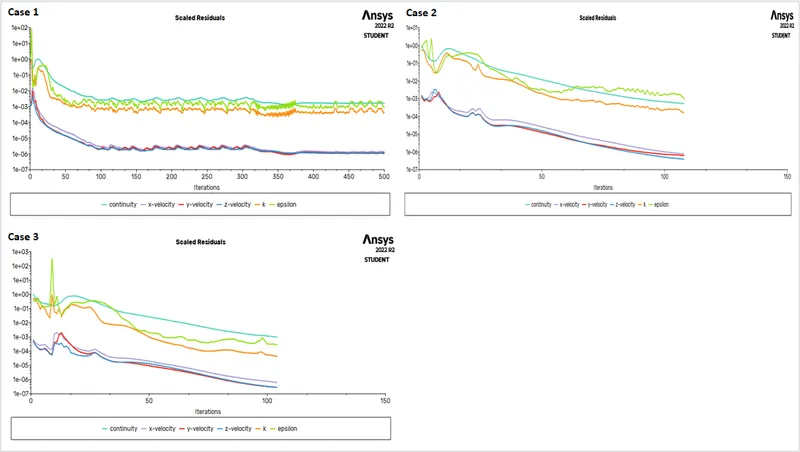
Scaled Residuals

Drag Plots

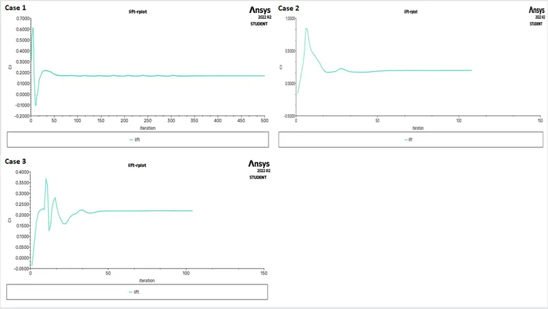
Lift Plots

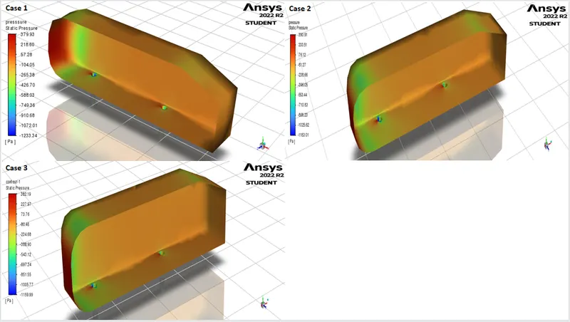
Pressure Contour on Car wall

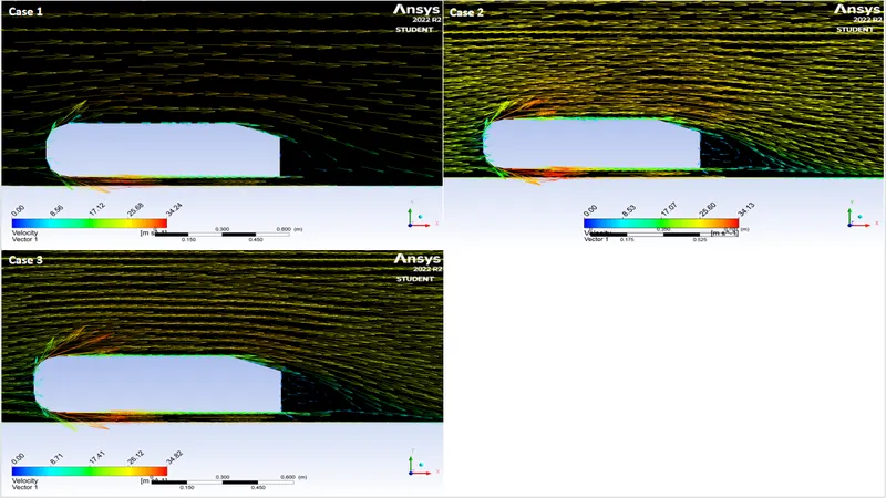
Velocity Vectors

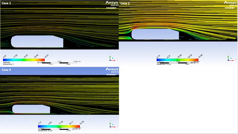
Velocity Streamlines

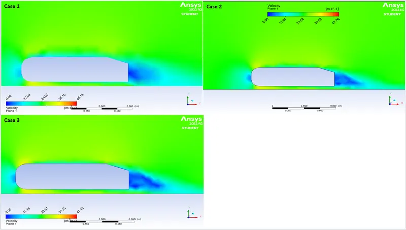
Velocity Contours

Distance from tail Vs Velocity Plots

Velocity vector at distance of 1.05 m, 1.5 m, 2 m and 2.5 m for case 1

Velocity vector at distance of 1.05 m, 1.5 m, 2 m and 2.5 m for case 2

Velocity vector at distance of 1.05 m, 1.5 m, 2 m and 2.5 m for case 3

CONCLUSION:

From the results of all 3 cases, let us tabulate for drag coefficient with respective grid sizes.

Grid Size	Case 1	Case 2	Case 3
Outer enclosure	250	100	80
Inner enclosure	100	50	45
Car wall	5	3	3
Drag coefficient	0.412	0.349	0.334
Lift coefficient	0.169	0.198	0.218

INFERENCES:

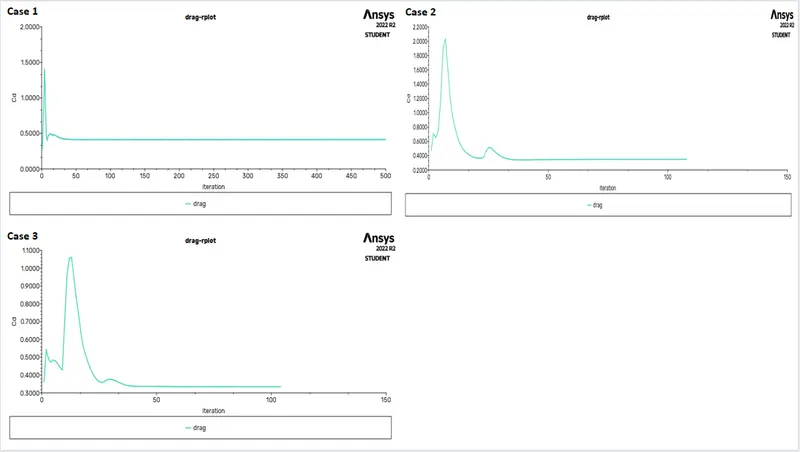
From the grid independency study, we come to know that the finer the mesh size the accurate the results. We have obtained the expected drag coefficient of 0.33 at the case 3.

As the drag coefficient decreases the lift coefficient increases

In the case 1 the solution is not really converged even after 500 iterations in coarse mesh, where as in case 2 and 3 in finer mesh the iterations are converged around 100 iterations itself. So, mesh size impacts the convergence as well.

From the velocity and pressure contours, the slant angle alpha of the rear face from the roof affects the wake region is observed.

The distance from the tail of car Vs Velocity plot shows that as the distance from tail increases the velocity is more stable due to the mixing of ambient upstream air. The same can be visualised in the form of slideshow animation provided in the results.

References:

CFD Simulation of Flow around External Vehicle: Ahmed Body Saurabh Banga1 , Md. Zunaid2*, Naushad Ahmad Ansari3 , Sagar Sharma4 , Rohit Singh Dungriyal5

IOSR Journal of Mechanical and Civil Engineering (IOSR-JMCE) e-ISSN: 2278-1684,p-ISSN: 2320-334X, Volume 12, Issue 4 Ver. III (Jul. - Aug. 2015), PP 87-94 www.iosrjournals.org