External flow simulation over an Ahmed body.
Introduction
The Ahmed body is a very generic and simplified model of a car. It was first developed by Ahmed and hence the name Ahmed body. A lot of work has been done on the Ahmed body, both computationally and experimentally. A wide variety and range of data for the Ahmed body are present in the form of literature. For this reason, and its simplicity, the Ahmed body is used as a basic test case to validate CFD codes.
Theory
Negative pressure regions and separation point
It is necessary to understand that the terminology negative pressure doesn't mean that the pressure is actually negative. The lowest pressure that can be achieved is the vacuum. Negative pressure in a region would mean that it has lower pressure than the surrounding region.
To understand the negative pressure more clearly and why it is developed, let us go through the following example.
Assume a stationary average car, there is air all around it at atmospheric pressure. Now when the car just starts to move forward, the air would flow from the front to the back of the car. There would be streamlined flow over the car. Now, when the flow reaches a separation point, i.e., where it can no longer maintain the streamlined nature, the flow leaves the surface.
The point where the flow leaves the surface is called the separation point. In scientific terms, it is the point where there is no more influence of the wall i.e., there is no zero wall shear stress. This flow with it would carry the air particles which were there behind the car when the car was at rest. So, the number of molecules behind the car has now considerably gone down, which implies the pressure has reduced. This is the negative pressure region that is developed behind the car.
Now since the pressure has gone down, naturally air from the high-pressure region should flow in and fill the void, ideally, this process starts and the flow tries to reverse in towards the car's moving direction. An interesting phenomenon is that if a car is moving right behind this car, then it would experience lesser pressure drag than if it were moving individually.
Wall Function
We generally provide the boundary condition for the body in the study as a no-slip condition. But how correct is it? It is only true if the flow is fully laminar. This is not the case in the current study. Here we use a turbulent model for solving the flow. In such cases, the boundary layer is sub-divided into different categories and the flow behaves differently in different sublayers. One such sub-layer is a very small highly viscous layer that can be treated as fully laminar; i.e., no-slip condition. This would mean that we would have to restrict the mesh size to capture the no-slip condition in the very first cell that is next to the boundary. The behavior of the flow would change from the very next cell. Without proper knowledge of the viscous sublayer thickness, it would require a very fine mesh for good results, which could rise the computational costs in multiple folds of magnitude.
There is something called a wall function that was developed to overcome this particular problem. A wall function helps the solver to understand and decide how to approach the solution near walls/boundaries. There are many wall functions used commercially. But the basic understanding is the same.
Here, we discuss a very basic and simple standard wall function. To understand it we must first familiarize ourselves with the terms shear velocity, y+ and y*.
Shear velocity which is sometimes also called frictional velocity is used to write shear-stress in terms of velocity. This is used to compare true velocities (flow velocities) with the velocities that relate to shear stresses between adjacent fluid layers.
`u_tau=root2(tau/rho)`
where `tau` is the shear stress and `rho` is the density.
y+ and y* are dimensionless numbers normal to the wall boundary. They are called y+ and y* no matter which direction is the normal of the wall facing.
Close to the boundary of the geometry, the viscosity and wall shear stress plays a major role, and thus the dimensionless numbers y+ and y* depend on them.
Experimental observations and Direct Numerical Simulations show that the fully developed flow has a universal shape (size is still scalable) when plotted along y+ or y* and u+, both being dimensionless numbers. It was also noted that the shape didn’t vary when the Reynolds number or the flow velocity was changed. This again is an advantage of using y+ and y*.
A y+ < 5, is within the Viscous sub-layer, a y+ > 30 is in the turbulent region and anything between the two must be avoided as the region is in a transition area or buffer area. In this region neither laminar nor log law gives good results, they both would lead to errors in the solution.
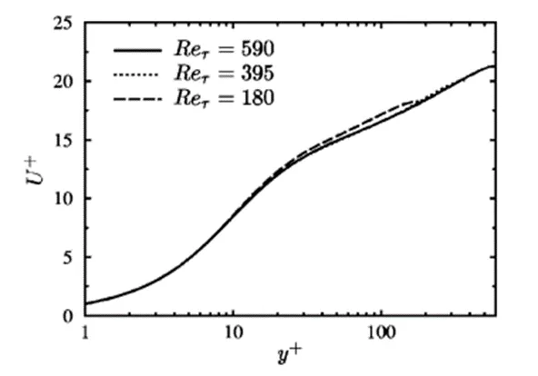
By calculating y+ or y*, finding the corresponding value for u+, and comparing it with the standard universal graphs, we can change the viscosity values near the wall so that the calculated and standard values match closely. This gives a well-developed flow profile as seen in experiments.
`y+=(rhoyu_tau)/mu` and
`ystar=(rhoyu_T)/mu`
where y is the distance from the wall.
What is the velocity to be selected? The velocity at the wall is zero, this would make the formula useless. The free stream velocity has a very less to negligible effect near the boundary layer, so using that also doesn’t make sense. Here, the sheer velocity discussed earlier comes into the picture.
`u_tau=root2(tau_w/rho)` and
`u_T=root2(c_mu^(1/2)k_p`,
where the value under the square root is the Turbulent Kinetic energy
The usage of the formula differentiates if y+ is being calculated or y*. Historically y+ was introduced first. The disadvantage of using y+ is that it uses more computational power as it involves iterations. Whereas y* does not have many iterations.
In flows with stagnation points or flow separations, the shear stress becomes zero or negative, this can cause problems while solving for y+. So, clearly, y* is more advantageous than y+.
But, y+ is a good indicator in cases of flow between parallel plates or flat surfaces. It is ideal to keep both y+ and y* under 5. It is best if they are close to 1.
Ansys fluent uses y* in its codes, whereas Open Foam gives an option to select between the two. Though Ansys uses y*in its codes, we can still compute y+ in the post-processing, this is done by using the wall shear stress and turbulent kinetic energy values from the solution. Generally, the values of y+ and y* are almost the same.
When a boundary in Ansys is specified as a wall, Ansys automatically applies the wall function on the specific boundary.
Pre-processing
Geometry
Tool - Ansys SpaceClaim
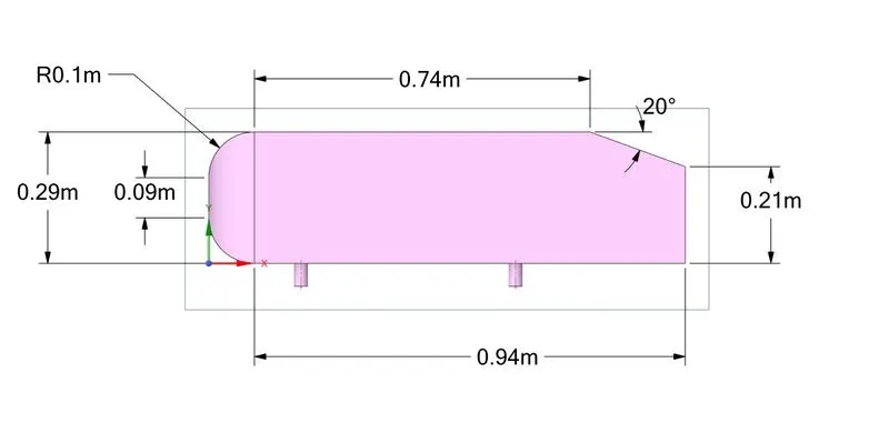
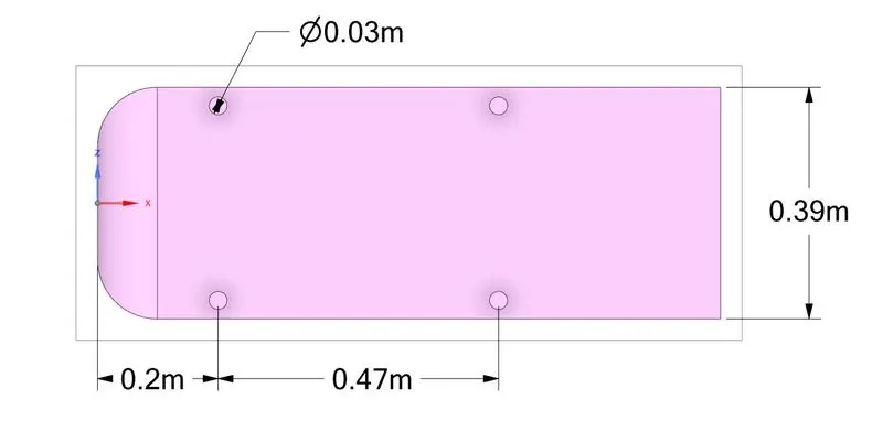
If the slant angle is < 12 degrees, the flow is attached and 2D, with low drag.
If the slant angle is between 12 degrees and 30 degrees, C pillar vortices are formed and the flow is 3D. The strength of these vortices is highest in the case of 30 degrees.
If the slant angle is greater than 30 degrees, then flow separation takes place, this results in a sudden decrease in frictional drag and weaker C-pillar vortices.
Dependence on Aspect ratio - As the aspect ratio of the slant increases, the critical angle decreases, this induces flow separation at lower angles.
- Since the body under study is a symmetric one, it is better to split it into two equal parts and delete one of them. This would save computational costs.
Enclosure
Enclosures are basically the flow fields. It is where the flow actually takes place. In this project, we create two enclosures, this is done to refine the area of study/interest or where the flow changes are highest.
Once this is done, always suppress the physics of the original geometry, as we will not require the mesh inside of the body. It is the surrounding area that is our focus.
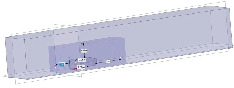
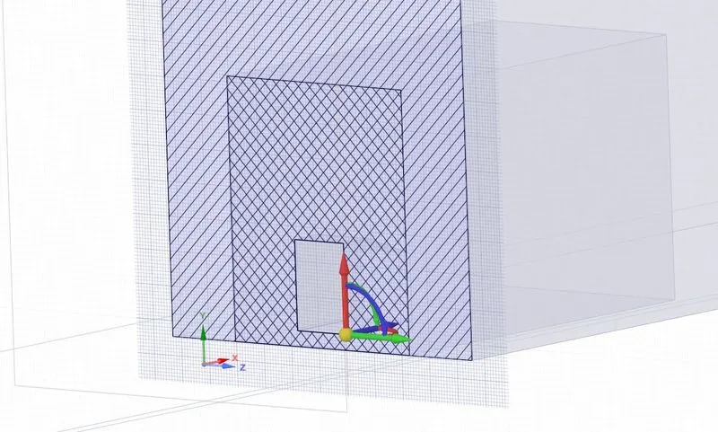
When these enclosures are sliced using cut planes as shown below, we can see that the hatching pattern overlaps with the other hatching patterns. This implies that there is interference between the enclosures and it has to be removed.
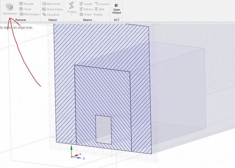
Once the interference is removed, split the enclosures, just like the Ahmed body was split.
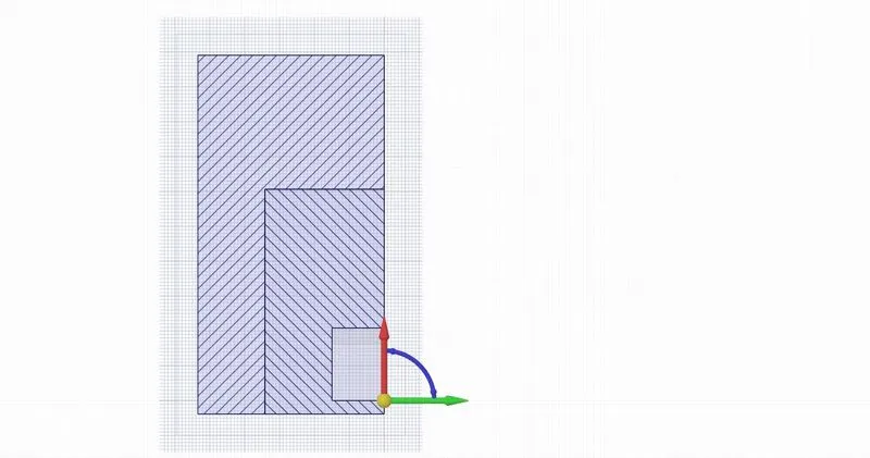
If the mesh is generated at this stage, the meshing wouldn't be continuous between the outer and inner enclosures, this might lead to gradient generations at these boundaries. This can be avoided by sharing topology between the enclosures as follows.
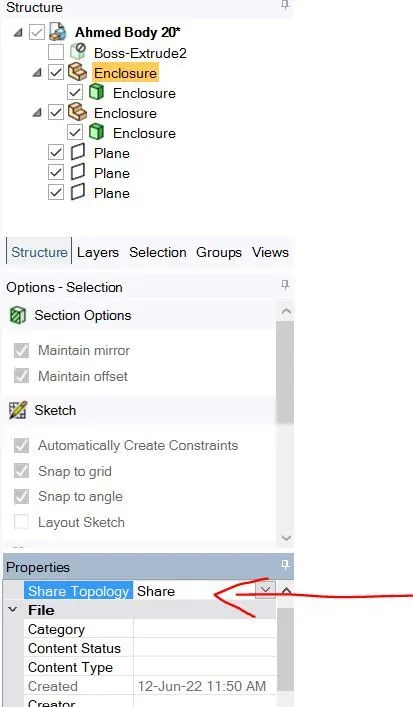
Repeat the step for the other enclosure also.
Topology sharing can also be done as follows.
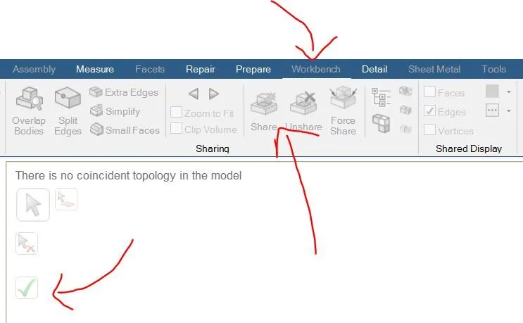
The geometry is fully ready for meshing
Meshing
1. Auto-generated Mesh
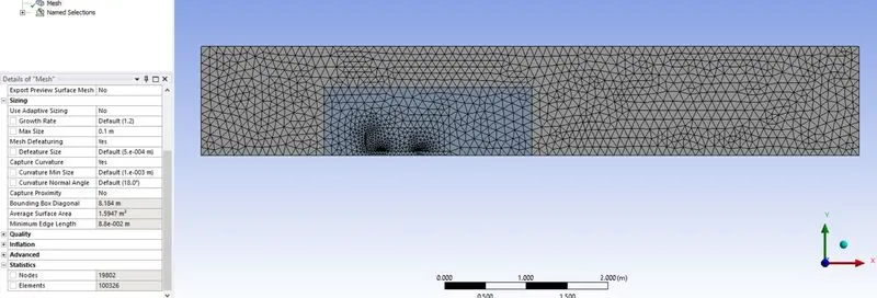
2.
Method = Multizone
Effectivity = Outer Enclosure
This improves the uniformity and makes the mesh more structured. Also, reducing the number of cells, thus reducing the computational costs.
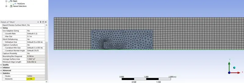
3.
Method = Body sizing
Effectivity = Inner Enclosure
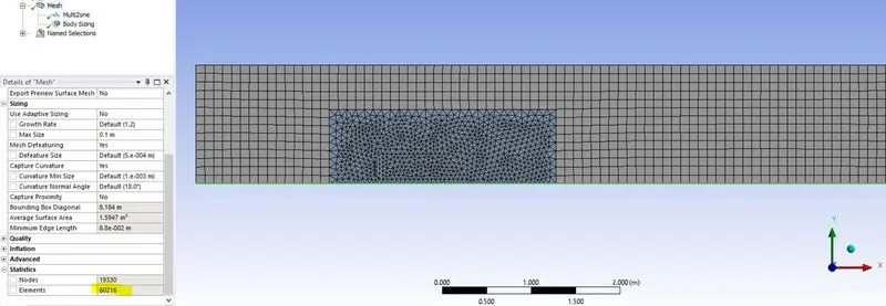
4.
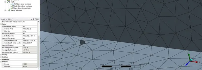
Method = Face sizing
Effectivity = Ahmed body
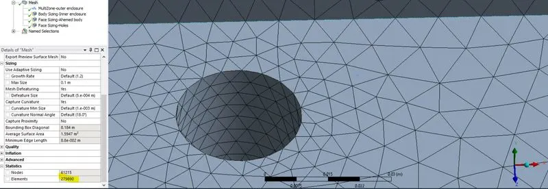
This is done hoping, that the cylindrical holes in the Ahmed body would get a circular boundary rather than the polygonal as shown in the following picture.
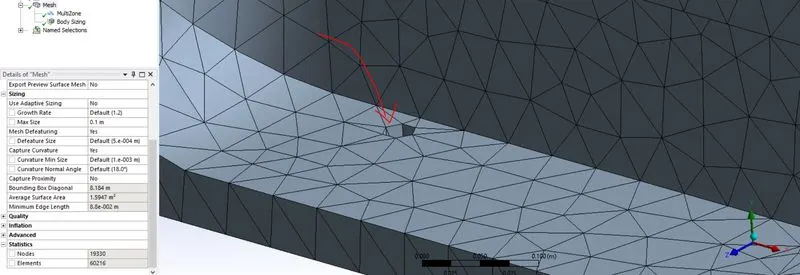
This method apparently didn't work and gave the following output.
5.
Method = Edge sizing
Effectivity = Cylindrical holes
Number of divisions = 36
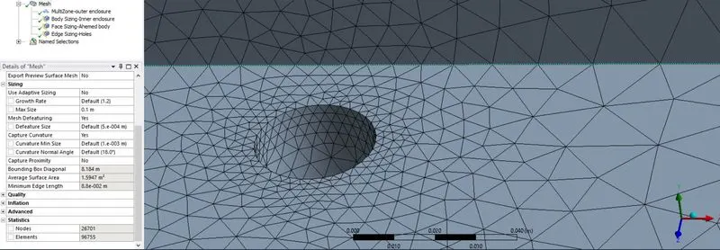
The mesh is still not refined on the cylindrical surface.
6.
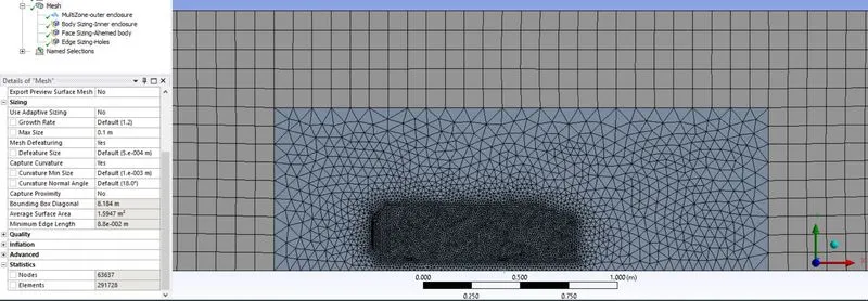
Method = Face sizing
Effectivity = Ahmed body
7.
The edge sizing of the holes is deleted.
Method = Face sizing
Effectivity = Cylindrical surfaces.
8.
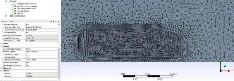
Method = Inflation layers
Effectivity = Boundary faces of the Ahmed body.
This is done in an attempt to incorporate the boundary cell's centroid in the Laminar sublayer or to make y+ < 10.
Setup
Flow characterisitcs
Material = Air
`rho = 1.225 kgm^-3`
`u=25ms^-1`
`L=1.0488m`
`mu=1.7894 ** 10^-5 kg(ms)^-1`
`Re=(rhouL)/mu`
`Re=1.225**25**1.0488/(1.7894**10^-5)`
`Re=1794987.14652`
Since the Reynolds number is too high, we use the turbulent model.
- Pressure-based solver (Reason = Incompressible flow)
- Method = SIMPLE
- Steady flow
- Turbulent model
- Viscous = k-omega SST (Reason = Captures physics both at boundary layer and away from boundary layer)
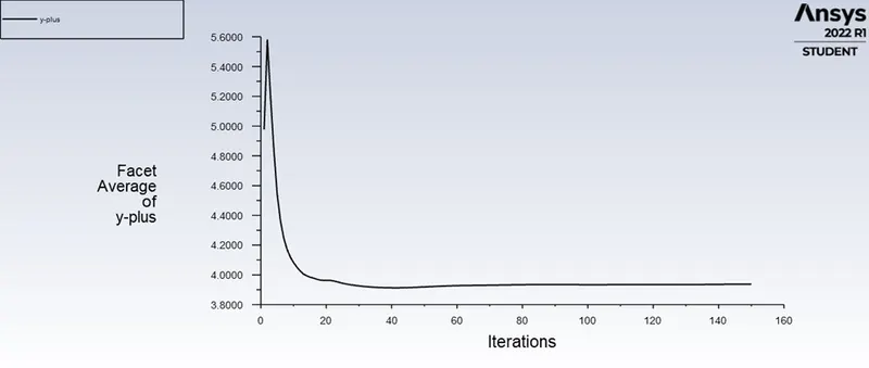
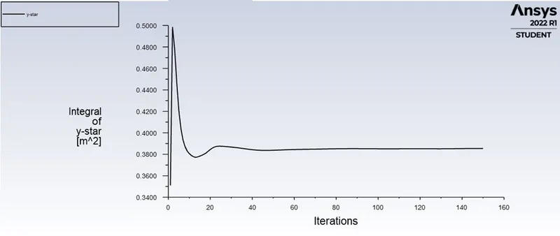
The solver is run and y+ and y* values are calculated and the plots obtained are as shown below.
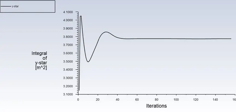
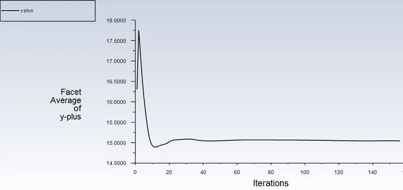
The value of y+ is 15 and it is not a very ideal value. It is always prescribed to avoid y+ values between 5 and 30. The y+ value can be reduced by reducing the size of the inflation layer at the faces of the Ahmed body,
Re-Meshing
Reduce the inflation layer size.
Type = First layer thickness
Value = 0.002
Create necessary plots, animations, and planes as necessary.
Post-Processing
y+ and y*
Both y+ and y* are under 10, which is a very good sign that the boundary cells are in the laminar sublayer and the no-slip condition holds good in such cells.
Convergence
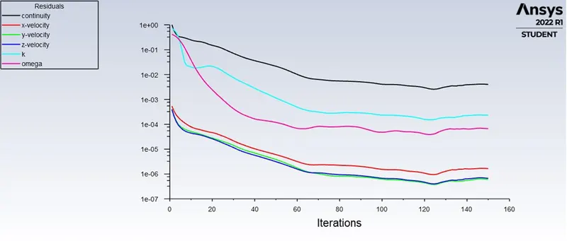
It is pretty much clear from the residuals that the solution has more or less converged.
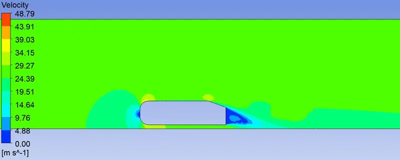
Velocity contours at the center and at the cross-sections where holes/wheels are present
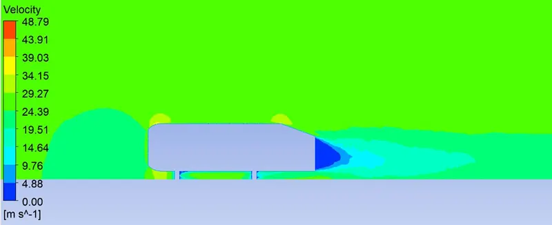
Observations
- Stagnation points are formed at the mid-section, but not close to the edges. This is acceptable, as the flow far from the mid section moves towards the sides and the streamline keeps moving. Hence, no stagnation points.
- The wake behind the body in the mid-section is like the trailing edge of an unsymmetrical airfoil, whereas the wake behind the body far from the mid-section is more like the trailing edge of a symmetric airfoil. I assume this is because the flow at the sides is more 3 Dimensional because of the high-pressure flow from the sides of the body moving in to fill the void behind.
- The high-velocity region near the slant start point can be a separation point, but the flow seems to reattach the slant soon.
Pressure contours at the center and at the cross-sections where holes/wheels are present
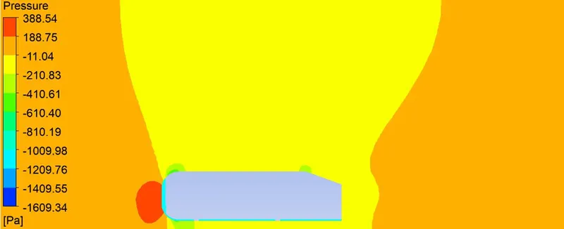
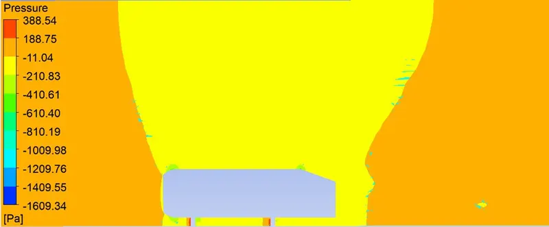
Observations
- Stagnation points in front of the body at the mid-section are the reason for high pressures in the specific areas.
- Stagnation points can also be seen at the wheel/leg location.
- All the other areas have negative pressure (in a relative sense)
Coefficient of Drag
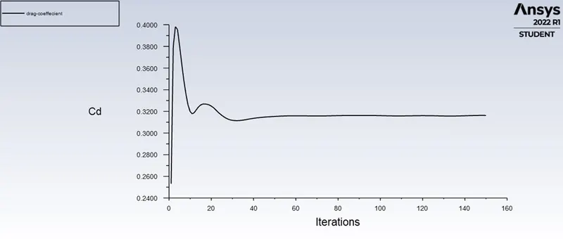
Observations
- The coefficient of drag was found to be 0.31626, which is close to the value cited in the literature i.e, 0.33
- The Cd value might get closer to the value cited in the literature if the mesh is further refined.
Wake visualization
Observations
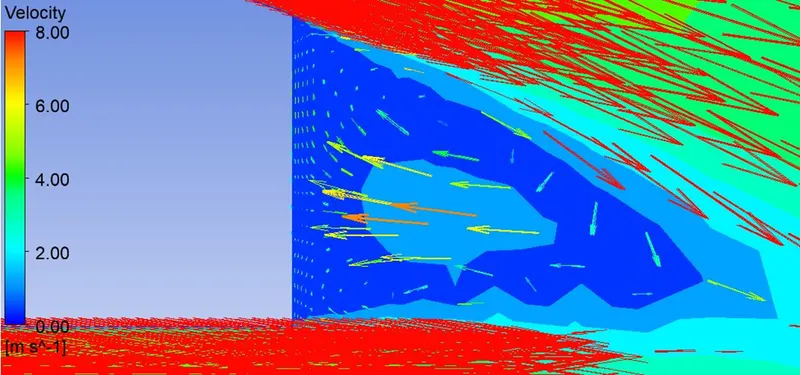
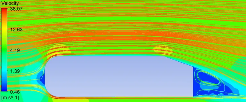
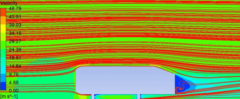
- The vectors and the streamlines clearly indicate that there is flow reversal due to low pressure behind the body. This is called as wake.
Grid Independence
| Cells | Lift Force | Drag Force | Coeff of Lift | Coeff of Drag | % change in Drag |
| 279198 | 0.31626 | ||||
| 316790 | 6.3215 N | 6.7401 N | 0.2947 | 0.3143182 | 0.614 |
| 354998 | 5.2957 N | 6.7246 N | 0.24696 | 0.31359 | 0.23167 |
| 466087 | 6.288 N | 6.5928 N | 0.2932 | 0.3074 | 1.97391 |
In all the above cases, even on further refinement of the mesh, the percentage change in the value of the drag coeffecient is not more than 2%. This implies that grid independence has been achived.
Conclusion
| Cells | Cd (CFD) | Cd (Experimental) | % Change |
| 279198 | 0.31626 | 0.33 | 4.16364 |
| 316790 | 0.3143182 | 0.33 | 4.75212 |
| 354998 | 0.31359 | 0.33 | 4.97273 |
| 466087 | 0.3074 | 0.33 | 6.84848 |
It has been concluded that the Cd obtained from computational methods is around 0.31, which is around 4-5 % lower than the value obtained in the literature.
References