Week 3 - External flow simulation over an Ahmed body.
AIM:- To simulate External flow over an Ahmed body using Ansys Fluent
Objective:-
- To simulate external flow over Ahmed's body and understand its importance.
- Calculate the numerical values for drag and lift coefficient and validate with analytical values.
- To perform Grid Independency test and compare error for drag and lift coefficient
Introduction-
Ahmed body is a generic car body (a simplified car model) i.e the flow of air around the Ahmed body captures the essential flow features around an automobile. The aim is to simulate the model on computational fluid dynamics (CFD) software(Ansys Fluent) and compare the Drag Coefficient, Velocity Profiles, Velocity field, and the time-averaged Wake structure of the CFD simulation results with the real experimental measurement in the wind tunnel.
Theory:-
Ahmed Body-
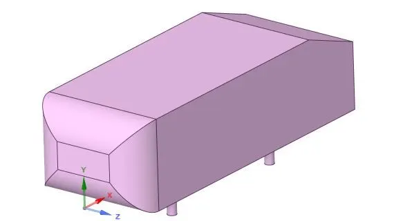
As the burning of fossil fuels becomes a more pressing issue, manufacturers are introducing more fuel-efficient cars to the market. One main contributor to fuel burn is the car’s aerodynamic drag. Complexly shaped, cars are very challenging to model and it’s difficult to quantify the aerodynamic drag computationally. The Ahmed body is a benchmark model widely used in the automotive industry for validating simulation tools. The Ahmed body shape is simple enough to model while maintaining car-like geometry features.
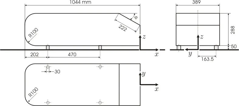
What Is an Ahmed Body?
The Ahmed Body was first created by S.R. Ahmed in his research “Some Salient Features of the Time-Averaged Ground Vehicle Wake” in 1984. Since then, it has become a benchmark for aerodynamic simulation tools. The simple geometrical shape has a length of 1.044 meters, a height of 0.288 meters, and a width of 0.389 meters. It also has 0.5-meter cylindrical legs attached to the bottom of the body and the rear surface has a slant that falls off at 40 degrees.
Modeling Airflow Over an Ahmed Body
In the Airflow Over an Ahmed Body verification model, our Ahmed body has a 25-degree slant and is placed in a flow domain that is 8.044 x 1.389 x 1.288 meters (length x width x height) the front of the body is placed at a distance of 2m from the flow inlet. To reduce the computational cost, the asymmetry plane is introduced to simulate half of the model.
The flow for this model is turbulent, which is based on the Reynolds number determined by the body length and inlet velocity.
| Characteristic Length (D) | 1.044 m |
| Fluid Velocity (V) | 25 `m/s` |
| Fluid Density (`rho`) | 1.255 `(kg)/m^3` |
| Fluid Viscosity Dynamic (`mu`) | `0.000017894 (kg) / (ms)` |
| Reynolds Number | `1.79 × 10^6` |
The simulation solves for the turbulent kinetic energy in addition to the velocity field. For this simulation, we need a larger mesh size than what is usually common to resolve the turbulent flow. More specifically, we use a finer mesh downstream of the model to capture the wake zone.
The Reynolds number based on the length of the body, L, and the inlet velocity is `1.79 × 10^6`, which means that the flow is turbulent. The k-ε turbulence model is applied to account for the turbulence.
Boundary Condition
Air enters the computational domain at a freestream velocity u∞ = 25 m/s normals to the inlet surface. At the outlet, a Pressure condition is applied. The floor of the flow domain and surface of the Ahmed body is described by wall functions. Wall functions could also be applied to the outer wall and the ceiling of the wind tunnel. Their main effect on the flow around the body is, however, to keep the flow contained; therefore it suffices to model these as slip walls. The temperature is assumed to be 293 K and the reference pressure is 1 atm.
Meshing
There are two important aspects of meshing. The first is to resolve the flow in the wake. To achieve this, additional mesh control entities are introduced in the geometry. These entities are advantageous to normal geometrical entities since they are removed once they have meshed. A smoothing algorithm then smooths the mesh locally in order to minimize gradients in the mesh size. Also, it is easier to introduce a boundary layer mesh when the control entities are removed.
Procedure-
Ansys Fluent as CFD software is used to solve for Ahmed body external flow.
Geometry-
Importing - The original CAD model of the Ahmed body is imported in SpaceClaim which was in the STEP file format. Original STEP files are usually too complex for comprehensive CFD simulations, so certain preprocessing (cleaning) CAD work is generally required.
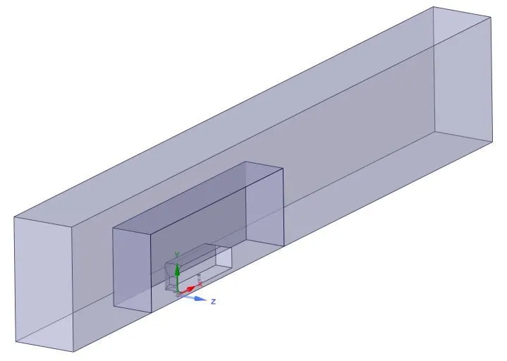
Creating Enclosure (Wind Tunnel)- A flow domain that is 8.044 x 1.389 x 1.288 meters (length x width x height) is created, the front of the body is placed at a distance of 2m from the flow inlet.
This acts as a Real-time wind tunnel for our computational solution.
Also, a small enclosure is then created around the model in order to capture the physics more accurately around the model.
Spilling the model - To reduce the computational cost, the asymmetry plane is introduced to simulate half of the model.
Mesh-
Boundary condition- First, we will name the face as inlet, outlet, symmetry, and car wall.
Inlet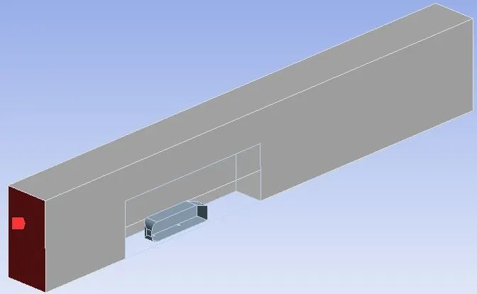 |
Outlet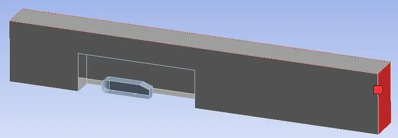 |
Symmetry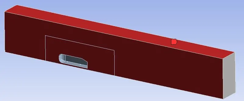 |
Car wall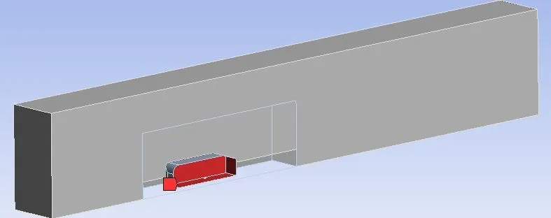 |
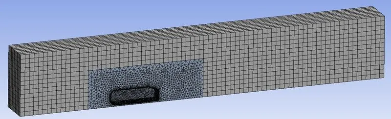
Mesh- We create our baseline mesh, then refine the mesh.
Setup-
Cases- In order to perform the simulation, we are interested in the final output, we will we using a Steady-state simulation with a K-epsilon turbulence model.
The cases are based on different Y+ values and varying mesh sizes.
| Cases | Y+ values | Mesh |
| Case 1 | 150 | 86275 - Course mesh |
| Case 2 | 150 | 138875 - Fine mesh |
| Case 3 | 70 | 432008 - Refind mesh |
Case 1-
- For the 1st case, Y+ is 150, and the K-epsilon turbulence model is used for study state simulation.
| Enclosure 1 Mesh size | Element size - 100mm (Hexahedral) |
| Enclosure 2 Mesh size | Element size - 50 (Tetrahedral) |
| Ahmed body Mesh size | Element size - 25 (Tetrahedral) |
| Y plus (Total Thickness) | 43mm |
| Number of Inflation Layer | 6 |
| Growth rate | 1.2 |
| Total number of cells | 86275 |
Meshing-
Outside Enclosure 1 with 100mm Hexahedral element
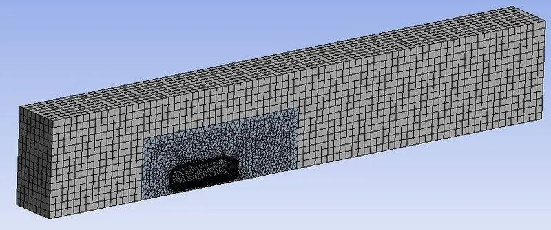
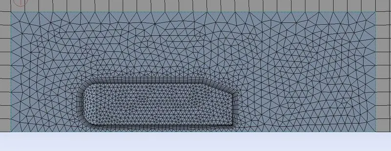
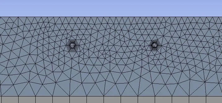
Enclosure 2 with 50mm Hexahedral element
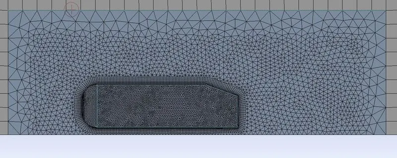
Ahmed's body has a Face sizing of 25mm with Tetrahedral mesh and 6 prism layers.
Results
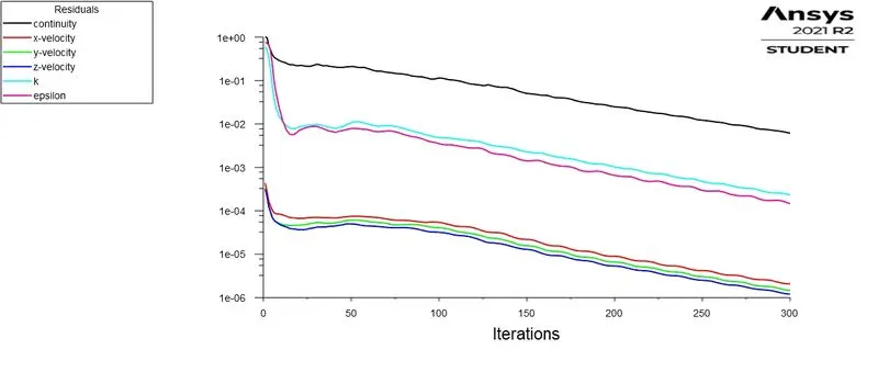
Residual graphs
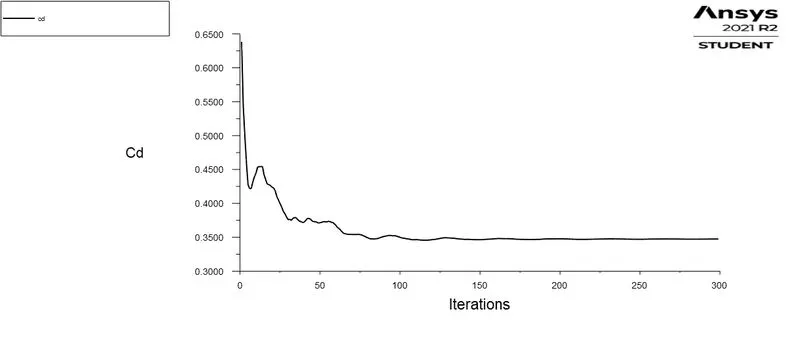
Coefficient of drag (cd)
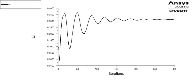
Coefficient of lift (cl)
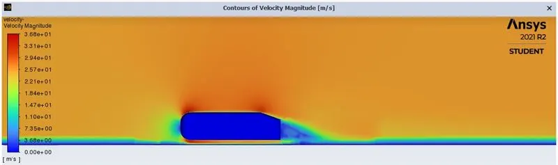
Contour plots
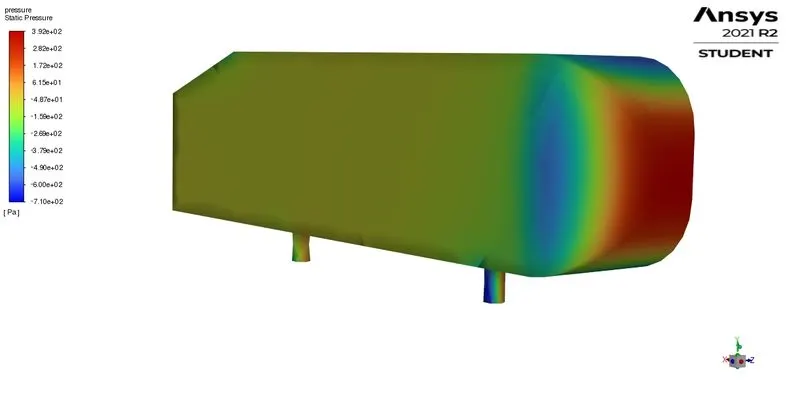
Pressure contour
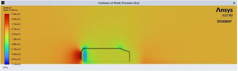
Pressure on Ahmed Body
Velocity Contour
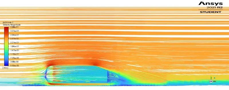
Velocity Pathlines
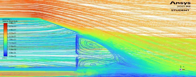
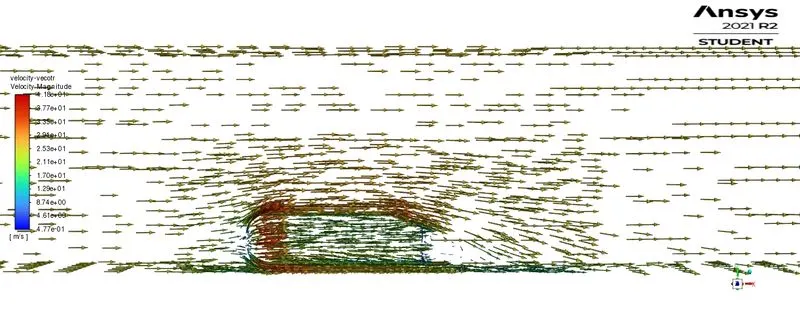
velocity Vector graph
Case 2-
- For the 1st case, Y+ is 150, and the K-epsilon turbulence model is used for study state simulation.
- In this case, as we are interested in the region near the wall so I have refined the mesh over the Ahmed body putting a face mesh size 15m
| Enclosure 1 Mesh size | Element size - 100mm (Hexahedral) |
| Enclosure 2 Mesh size | Element size - 50 (Tetrahedral) |
| Ahmed body Mesh size | Refined Element size - 15 (Tetrahedral) |
| Y plus (Total Thickness) | 43mm |
| Number of Inflation Layer | 6 |
| Growth rate | 1.2 |
| Total number of cells | 138875 |
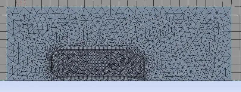
Meshing-
Outside Enclosure 1 with 100mm Hexahedral element
Enclosure 2 with 50mm Hexahedral element
Ahmed's body has a Face sizing of 25mm with Tetrahedral mesh and 6 prism layers.
Results
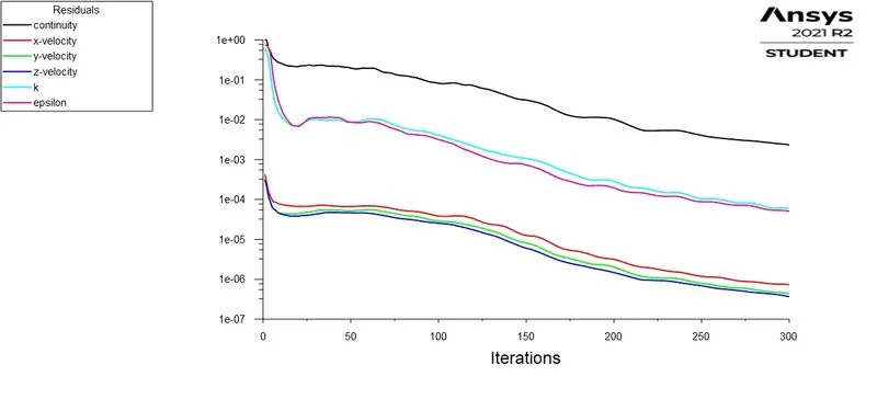
Residual graphs
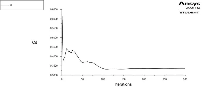
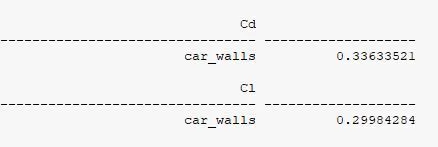
Coefficient of drag (cd)
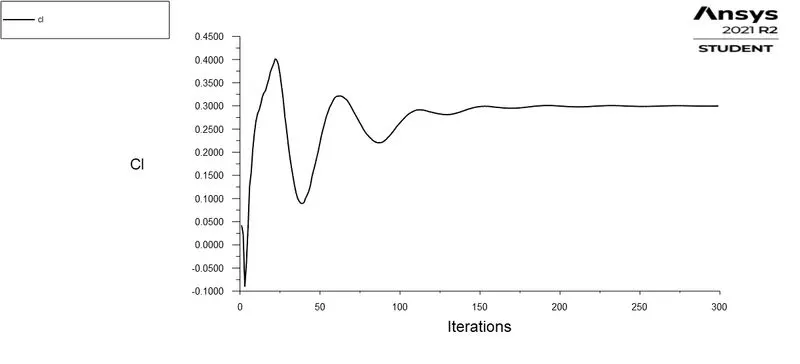
Coefficient of lift (cl)
Contour plots
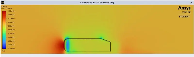
Pressure contour
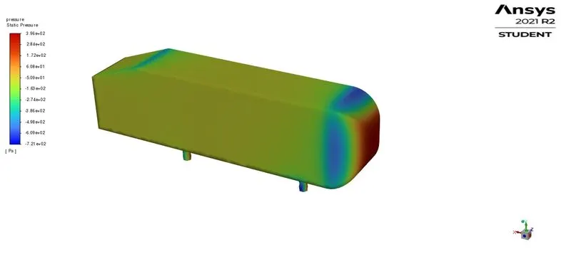
Pressure on Ahmed Body
Velocity Contour
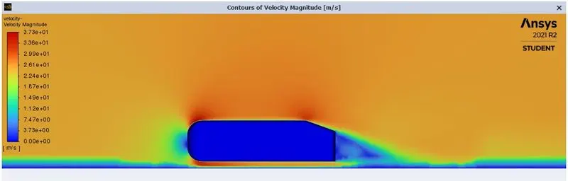
Velocity Pathlines
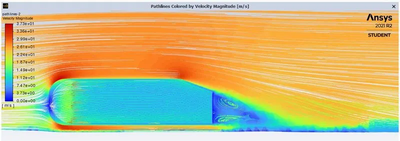
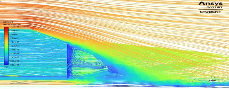
velocity Vector graph
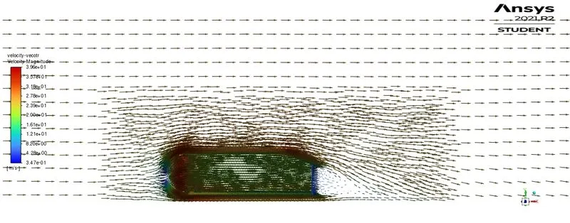
Case 3-
- For the 1st case, Y+ is 150, and the K-epsilon turbulence model is used for study state simulation.
- In this case, I further refined the mesh in order to get more accurate results.
| Enclosure 1 Mesh size | Element size - 100mm (Hexahedral) |
| Enclosure 2 Mesh size | Element size - 30 (Tetrahedral) |
| Ahmed body Mesh size | Element size - 10 (Tetrahedral) |
| Y plus (Total Thickness) | 53mm |
| Number of Inflation Layer | 10 |
| Growth rate | 1.2 |
| Total number of cells | 432008 |
Meshing-
Outside Enclosure 1 with 100mm Hexahedral element
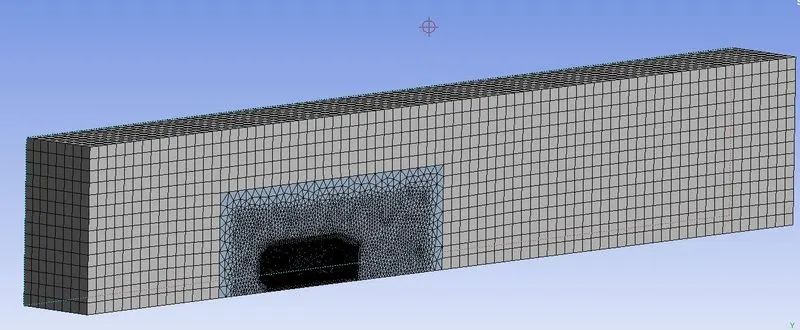
Enclosure 2 with 50mm Hexahedral element
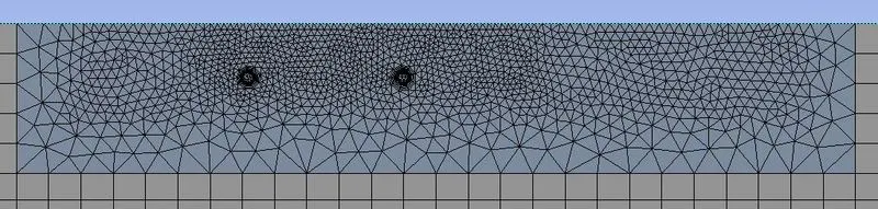
Ahmed's body has a Face sizing of 25mm with Tetrahedral mesh and 6 prism layers.
Results
Residual graphs
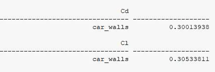
Coefficient of drag (cd)
Coefficient of lift (cl)
Contour plots
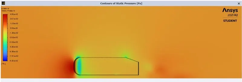
Pressure contour
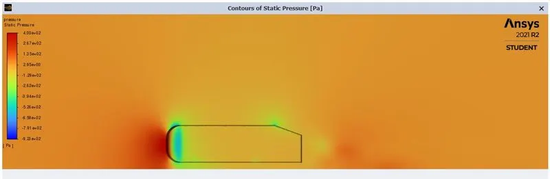
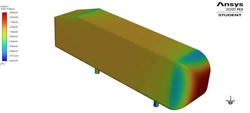
Pressure on Ahmed Body
Velocity Contour
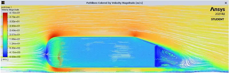
Velocity Pathlines
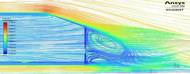
Velocity Vector Graph
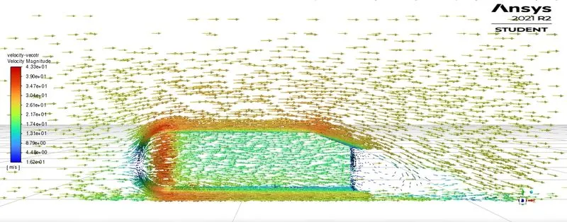
Observation From the cases (Grid Independency)
| Cases | Number of cells | Y+ | Analytical Drag Coefficient (Cd) | Drag Coefficient (Cd) | Lift Coefficient (Cl) |
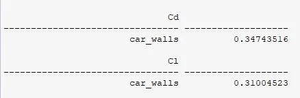
| Case 1 | 86275 | 150 | 0.311 | 0.3474 | 0.3100 |
| Case 2 | 138875 | 150 | 0.311 | 0.3363 | 0.2998 |
| Case 3 | 432008 | 100 | 0.311 | 0.3001 | 0.3053 |
Below are the Analytical values for Drag Coefficient on Varying Renold's number.
- The Standard Drag Coefficient is taken from the experimental data by W.meile
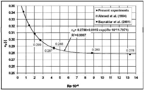
So for our case as Renold's number is Re = 1786772, the drag coefficient = 0.0311 (is approx)
Explanation of the terms
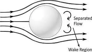
Point of separation- Point of separation forms at the rear end of the vehicle where drag is generated in the wake region.30 degrees is the critical angle of slant where separation occurs. Point of separation is a highly undesirable phenomenon and can be delayed in turbulent flows. The point of separation also depends on the shape and orientation of the body. Because of flow separation, low-pressure region forms were at some specified conditions where even vortex shedding can occur.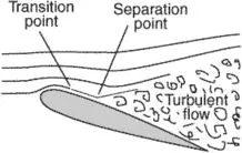
Flow Separation - The presence of the fluid viscosity slows down the fluid particles very close to the solid surface and forms a thin slow-moving fluid layer called a boundary layer. The flow velocity is zero at the surface to satisfy the no-slip boundary condition. Inside the boundary layer, flow momentum is quite low since it experiences a strong viscous flow resistance. Therefore, the boundary layer flow is sensitive to the external pressure gradient (as the form of a pressure force acting upon fluid particles). The pressure is increasing in the direction of the flow, an adverse pressure gradient condition as so it is called exist. In addition to the presence of a strong viscous force, the fluid particles now have to move against the increasing pressure force. Therefore, the fluid particles could be stopped or reversed, causing the neighboring particles to move away from the surface. This phenomenon is called the boundary layer separation.
Negative pressure in the Wake Region- Consider a fluid particle flows within the boundary layer around Ahmed's Body. The pressure is a maximum at the stagnation point and gradually decreases along the slant angle. The flow stays attached in this favorable pressure region as expected. However, the pressure starts to increase in the rear side of the body and the particle now experiences an adverse pressure gradient. Consequently, the flow separates from the surface and creates a highly turbulent region behind the Ahmed body called the wake. The pressure inside the wake region remains low as the flow separates and a net pressure force (pressure drag) is produced.
In general, it is considered that when air is removed from a region then a vacuum is generated in that region. If the particles in the wake still striking(colliding) with some momentum on the rear face of the vehicle then they are actually pushing the vehicle forward but why the force is considered to be opposing the motion (for example if the vehicle is moving along -ve X-axis then force in the wake is considered to be acting along +ve X-axis. Well, this is what we have observed during simulating the flow on vehicles.
Conclusion-
- The total drag coefficient of the Ahmed body is the key measurement for this simulation. It is made up of measurements for the pressure coefficients in the front, slant, and base of the body as well as the body’s skin friction. In the results of our simulation, the total drag is very well predicted but the individual measurements deviate from the experimental results in varying amounts.
- A few different factors cause these deviations in data. For the front and roof of the body, wall functions used in the simulation aren’t effective at predicting the flow transitions observed in the experiments.
- Here in this External Aerodynamic simulation it is important to refine the mesh near the wall and behind the body in order to get an accurate result.
- Although the data have quantitative differences, it is qualitatively equal to experimental results because the total drag coefficients are so close. There may be deviating details in the smaller data but the simulation still captures the major features of the flow over an Ahmed body. This simulation is more than adequate for calculating the overall drag coefficient.