Week 3 - External flow simulation over an Ahmed body.

AIM: To simulate the external flow simulations over an Ahmed body.

OBJECTIVE

• To describe Ahmed's body and its importance.
• To explain the reason for the negative pressure in the wake region.
• To explain the significance of the point of separation.

Expected Results:

• Velocity and pressure contours.
• The drag coefficient plot for a refined case. ( For velocity of 25m/sec, the drag coefficient should be around 0.33).
• The vector plot clearly showing the wake region.
• Perform the grid independency test and provide the values of drag and lift with each case.

INTRODUCTION

• Ahmed body is a generic car-type bluff body that is used as a reference model for simulation.
• It provides reference with lot of available experimental and numerical data to test the flow type generally found in cars,i.e, vortices downstream of body,flow separation, ground interaction etc.
• Prior going for detailed analysis with an actual car-geometry this model helps in validating cfd codes.
• These findings can be later used for improving the dewsign of real vehicles.

• It has three important parts:

(a) Front face (wind-ward face with rounded corners) adapts the flow in the inlet and

allows the boundary layer to follow the body shape without separation.

(b) a rectangular shape to stabilze the flow

(c) An area characterized by the slant angle, where the largest flow separation point is

located.

SOLVING AND MODELLING APPROACH

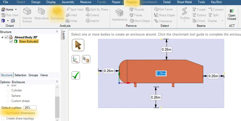
Fig. 1 1st enclosure around the geometry

• For simulating the external flow, we need to create an enclosure for making wind tunnel. To do so, in space-claim we have to select prepare -> enclosure and make sure to uncheck symmetric dimensions.
• Then we are able to edit the dimensions as shown in the above fig.1

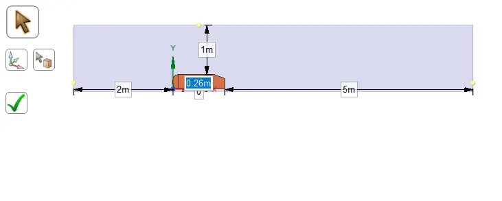
Fig. 2 distance measured from left,right ,top and bottom face of enclosure

• The above figure shows the dimensions of left,right,top and bottom surface of enclosure from ahmed body surface.

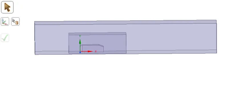
Fig. 3 Final geometry having two enclosure

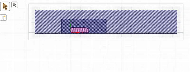
Fig. 4 Geometry depicts interference

• In geometry part we have two enclosure, so it better to check for interference as the mesh overlaps near interference region.
• We have to correct the interference if exist.In our geometry the interference is found and then it sis corrected.

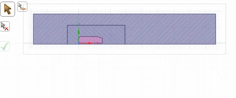
Fig. 5 Interference corrected

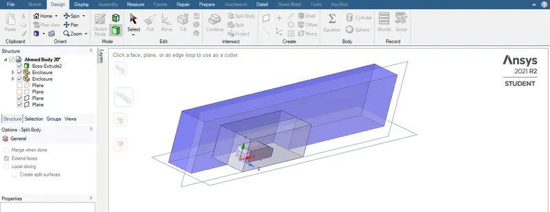
Fig. 6 Geometry is splitted using split body command in design tab

• In order to reduce the computation time ,we need to reduce the element size by splitting the body into equal parts,as the geometry is symmetry ,so we can use the 'split body', command in the design tab.
• We have to select body (outer encloser) first and then select cutter command to cut the geometry by selecting the XY plane.

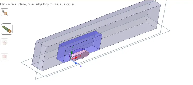
Fig. 7 Second enclosure is splitted using split body command

• The inner encloser is splitted by using the same procedure we did for the outer encloser.
• After that Ahmed body is splitted and the final geometry is transported to Ansys mesh.

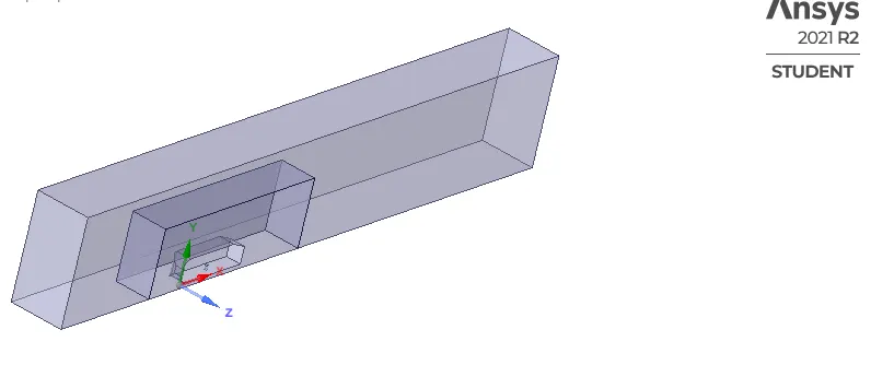
Fig. 8 Half of the geometry is splitted

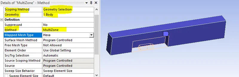
Fig. 9 creating hexahedral mesh where possible ( Multi-zone mesh method)

• For refining the mesh, the mesh methods are Multizone, body-sizing and Face sizing has been used.
• As shown in the fig., the mesh for selected part of geometry is hexahedral where possible to generate more accurate data.

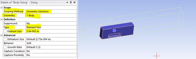
Fig. 10 Body sizing (Mesh refinement)

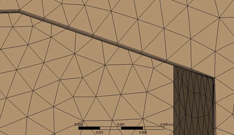
Fig. 11 inflation layers near car-wall surface

• Inflation layer is given on the car-wall for getting information of aerodynamic drag coefficient so that we can design the geometry for reducing the drag force where it is necessary.
• The total thickness of inflation layer merely depends on Y-plus value. For high reynolds number flow over bodies, it is generally taken as 50-300 as Y-plus value.
• Also we are able to get the body-fitted mesh as and when we are applying inflation layer.

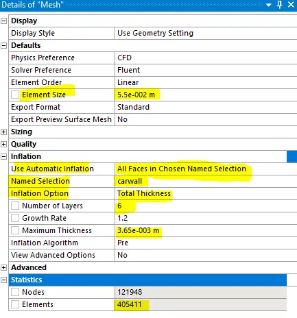
Fig. 12 Details of Mesh (number of elements has to be varied)

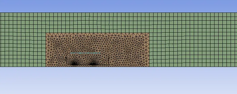
Fig. 13 Mesh element size of 100mm

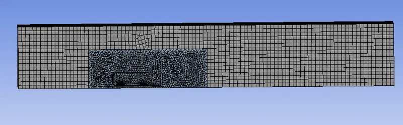
Fig. 14 Mesh element size of 80mm

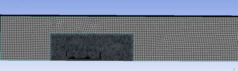
Fig. 15 Mesh element size of 55mm

Calulation of `Y^+`

• Dynamic viscosity of air @ 25deg celcius = 1.849*`10^(-5)` kg/(m.s)
• Density of air = 1.225 kg/`m^3`
• length =1.044 m
• Reynold's number= `(rho*velo*L)/(mu)`

Re= 1.225*25*1.044/(1.849*10^(-5) =`1.7*10^(6)`

Friction coefficient (`C_f`)=0.026/`Re^(1/7)`= 0.026/7.7636 = 0.00334

Wall shear (`tau_w`) = `(C_f*rho*v^2)/2`) = 0.00334*1.225*25*25 =1.2785

shear velocity (`mu_f`) =`sqrt(tau_w/rho`) =1.0216

Y= `(Y^+ *mu)/(rho*mu_f`) = 0.001477 taking Y plus as 100

Total thickness =`Y*(1.2^(N-1))` = 3.65mm where N= number of inflation layer=6

Y plus	Y	total thickness
80	0.00118mm	2.93mm
100	0.00147mm	3.65mm
120	0.00177mm	4.40mm
150	0.00221mm	5.49mm
200	0.00295mm	7.34mm

PRE-PROCESSING AND SOLVER SETTING

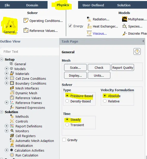
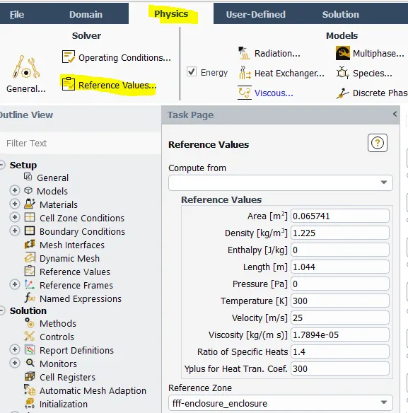
Fig. 16 setting up the physics and reference values

• for setting up the physics,pressure -based solver is used.As the Mach number is less than 0.3 (say) the compressibilty effect is neglected.
• We are interested in finding out the drag coefficient , lift -coeffiecient and wake formation behind the geometry, so steady state is used.

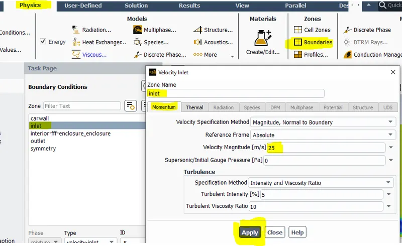
Fig. 17 setting up the boundary condition

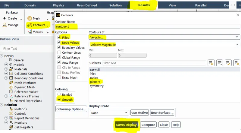
Fig. 18 Creating velocity contour

• After hybrid initialization we need solution animation to view the velocity variation over the surface of geometry.To do so,we need to create velocity contour along the flow field.

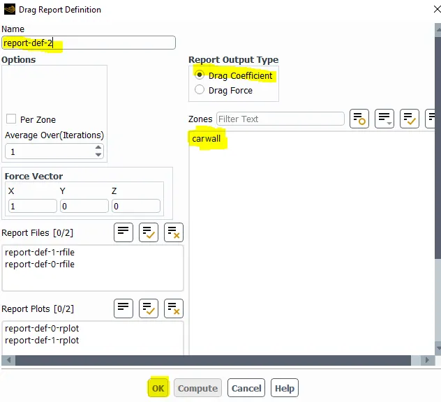
Fig. 19 Generating Report defination

• Report defination include drag coefficient, lift coefficient and drag force needs to be created for the analysis purpose i.e, CFD post processing results.

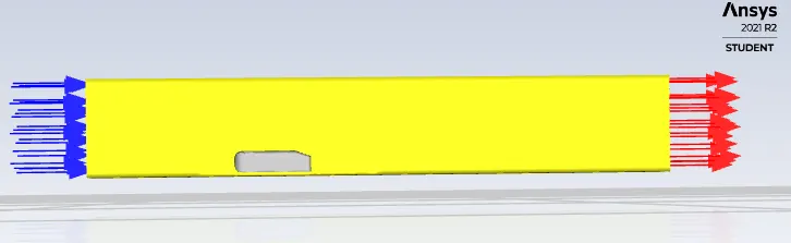
Fig. 20 Mesh is succesfully transported to fluent showing inlet and outlet perfectly

General set up boundary

Solver type : pressure-based

Turbulent Model: k-omega SST ,k-epsilon

Fluid Material : Air

Boundary condition

inlet :inlet velocity

outlet: outlet gauge pressure 0 Pa

side-wall: symmetry

RESULTS

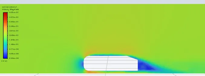
Fig. 21 velocity animation plot ( mesh size 100mm)

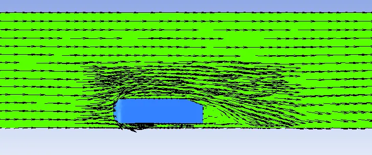
Fig. 22 Vector contour plot ( mesh size 100mm)

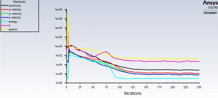
Fig. 23 Residual vs iterations ( mesh size 100mm)

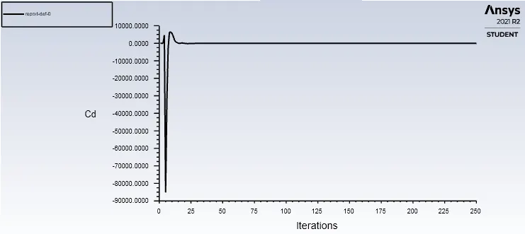
Fig. 24 Drag coefficient ( mesh size 100mm)

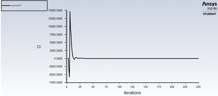
Fig. 25 lift coefficient ( mesh size 100mm)

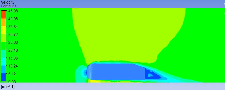
Fig. 26 Velocity contour plot ( mesh size 100mm)

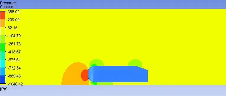
Fig. 27 pressure contour plot ( mesh size 100mm)

element size 80 mm, k-omega

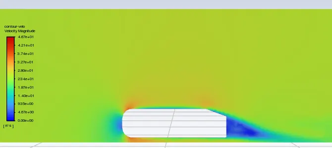
Fig. 28 velocity animation plot ( mesh size 80mm)

• When the mesh element size is refined ,we are getting the perfect low pressure region behind the ahmed body.
• The pressure at front is maximum and it is validated as the velocity is lower (stagnation point). Then the dynamic pressure decreases as shown in the figure with red color.

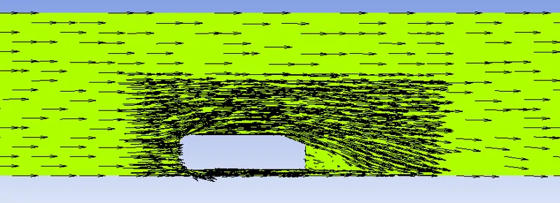
Fig. 29 Vector contour plot ( mesh size 80mm)

• Recirculation and vorticity is observed at rear side of the body, which depicts the drag is generated and suction pull is created forming the region low relative pressure zone.

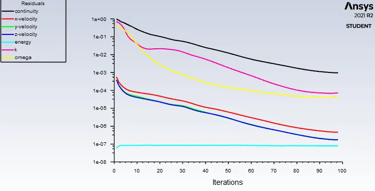
Fig. 30 Residual vs iterations ( mesh size 80mm)

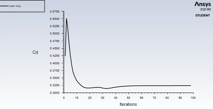
Fig. 31 Drag coefficient ( mesh size 80mm)

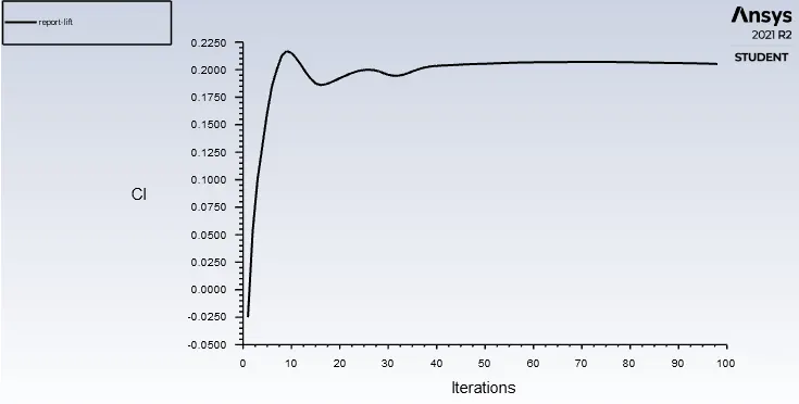
Fig. 32 Lift co-efficient ( mesh element size 80mm)

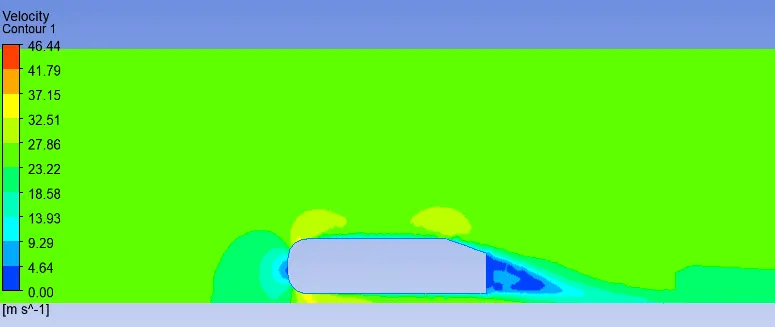
Fig. 33

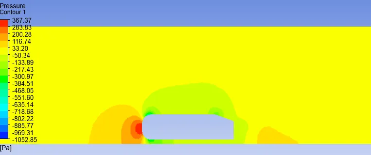
Fig. 34

element size 60mm, k-omega

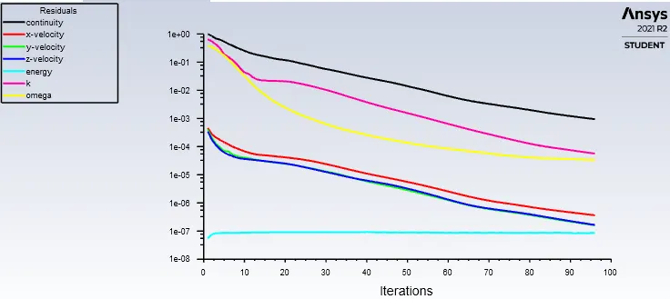
Fig. 35 Residual vs iterations ( mesh element size 60mm)

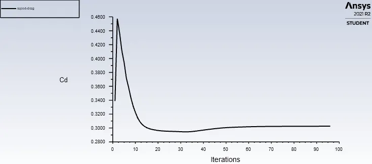
Fig. 36 Drag co-efficient ( mesh element size 60mm)

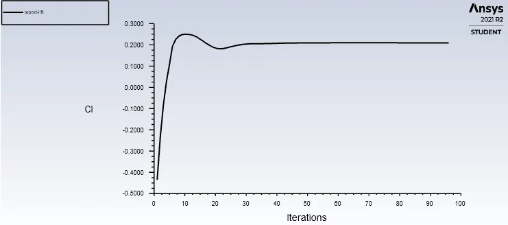
Fig. 37 Lift co-efficient ( mesh element size 60mm)

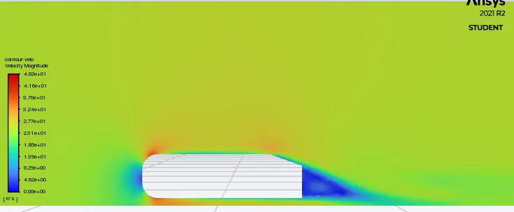
Fig. 38 Velocity animation plot ( mesh element size 60mm)

• The mesh element size is further refined, we are getting more appropriate result as we are able to capture the circulation zone and also the separation point just at the begining of slant surface .
• At the point of separation , if we look more precisely the blue colour depicts the low velocity ,it means the pressure at this surface is maximum compared to its previous surface. So adverse pressure gradient is created and flow field is separated.

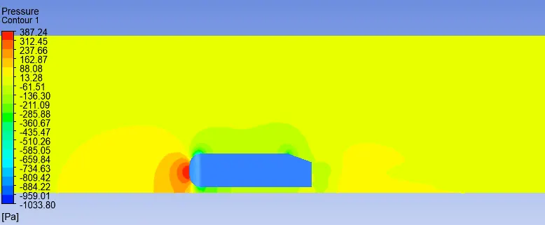
Fig. 39 Pressure contour plot ( mesh element size 60mm)

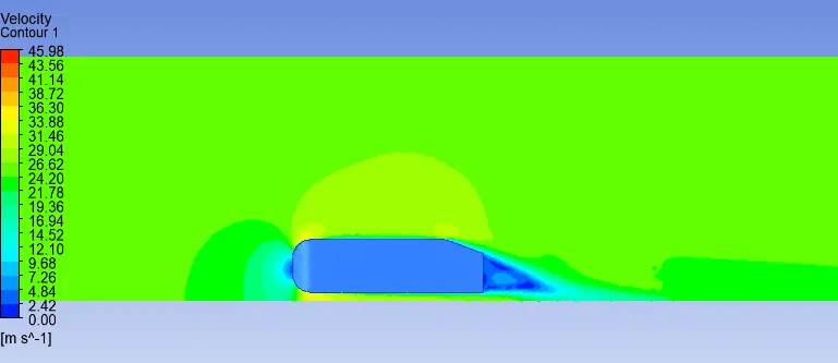
Fig. 40 Velocity contour plot ( mesh element size 60mm)

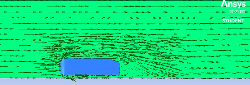
Fig. 41 Vector plot showing flow around Ahmed body ( mesh element size 60mm)

element size 55mm,k-omega

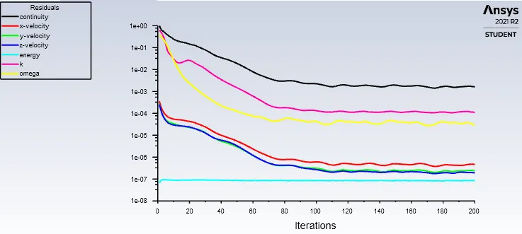
Fig. 42 Residual vs iterations ( mesh element size 55mm)

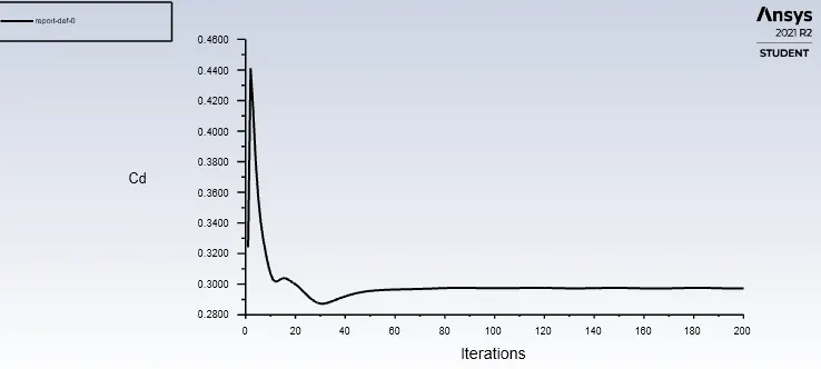
Fig. 43 Drag co-efficient ( mesh element size 55mm)

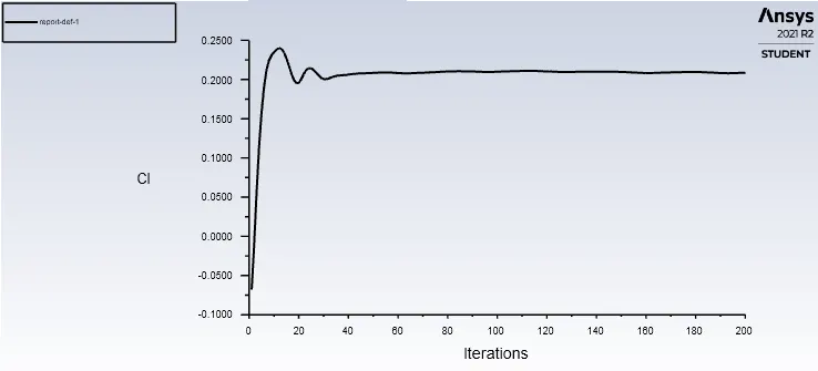
Fig. 44 Lift coefficient ( mesh element size 55mm)

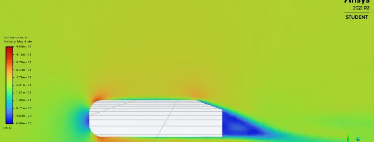
Fig. 45 Velocity animation plot ( mesh element size 55mm)

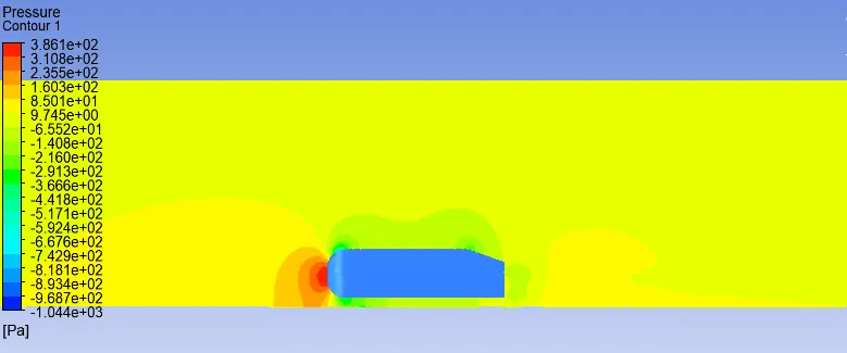
Fig. 46 Pressure contour plot ( mesh element size 55mm)

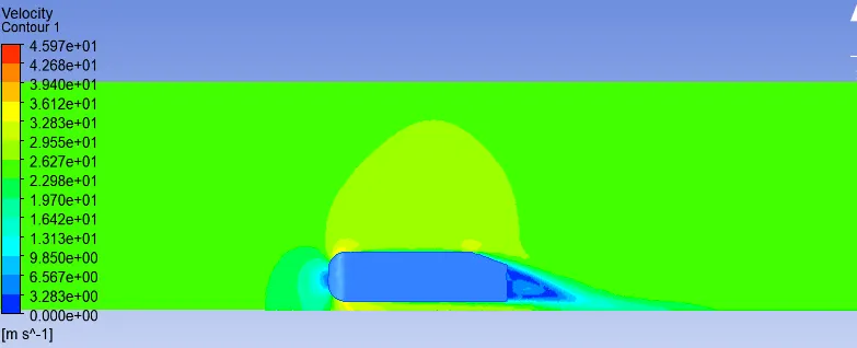
Fig. 47 Velocity contour plot ( mesh element size 55mm)

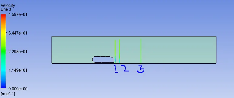
Fig. 48 line drawn downstream of plane of ahmed body to capture velocity profile

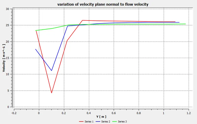
Fig. 49 Variation of velocity, plane normal to flow velocity ( mesh element size 55mm)

• In this graph, it is cleary visible that the velocity flow field above the geometry surface facing no disturbances and the there is no dissipation of energy.
• so far as flow near the geometry is considered , the shear layer coming from the top ,side and bottom surface generates vorticity(fluid rotating) resulting in turbulent eddies and energy is dissipated due to viscous effects .so the velocity decreases in the rear part of the geometry(ahmed body).
• When flow reattaches the velocity again increases as shown in the figure .

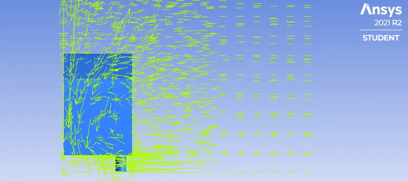
Fig. 50 vector plot showing ciculation ( mesh element size 55mm)

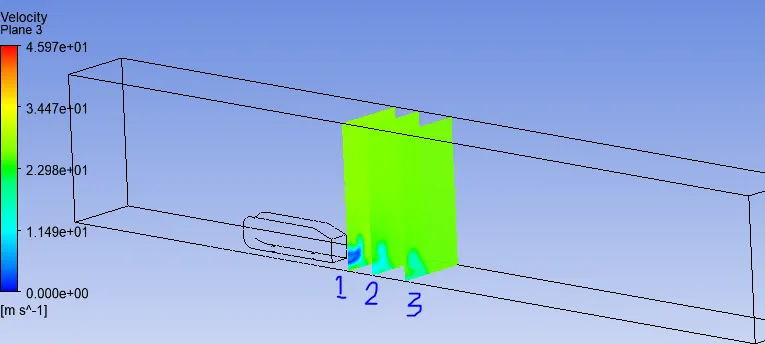
Fig. 51 Three planes are taken for capturing velocity profile at downstream of body

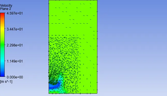
Fig. 52 Vector plot showing circulation at plane 1 ( mesh element size 55mm)

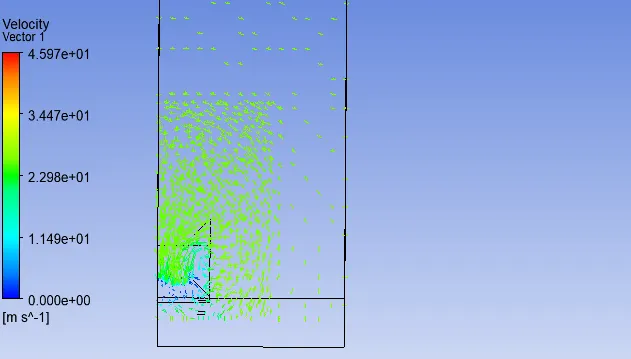
Fig. 53 Vector plot showing circulation at plane 2 ( mesh element size 55mm)

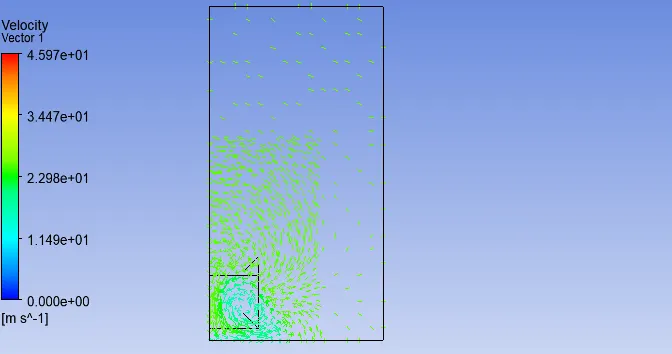
Fig. 54 Vector plot showing circulation at plane 3 ( mesh element size 55mm)

Reason for negative pressure in wake region

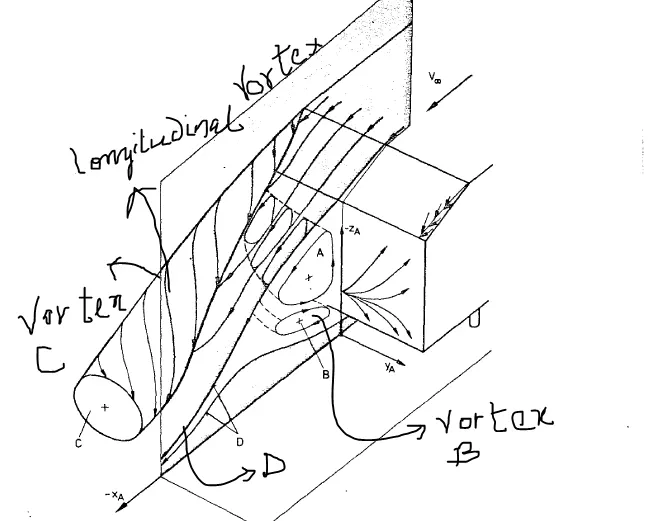
Fig. 55

• The higher flow velocity over the Ahmed body results in a lower pressure than under the vehicle body, wher the flow velocity is low. So, there is high pressure below the car and low pressure above the car surface.
• According to potential flow theory( which can be used to describe the flow outside the boundary layer), the pressure difference between between topside and bottomside of the car leads to circulation and lift force.
• The presence of circulation implies vorticity and it has to be preserved, so there wil be two trailing vortices from two side edges.
• The shear layer coming off the slant side edge rolls up into vortex and the shear layer rolls up into two recirculating flow regions 'A' and 'B' at the rear flat face having side top and bottom edge.

• The velocity at top surface is higher than at bottom surface. Near the surface ,the fluid particle comes to hault (no-slip boundary condition) and shear flow naturally creates angular momentum or vorticity.
• As the angular momentum accumulates , an an instability develops ,partially lifting the vortices above the wall.
• As we know the velocity above the wall(far from wall) is faster resulting in stretching and eventually the breaking up of the voetices into small segments.
• These vortices are now responsible for the perturbation of velocity vector in other direction.
• Thus ,more momentum is lost inturbulent flow (larger friction) but diffusion is enhanced.

• As the flow separates in the slant surface and reverse flow takes place, there is formation of vortices due to more relative pressure(at trailing edge) as compared to leading edge surface.
• Thus creating turbulent eddies and resulting in high velocity but the region near to rear surface suction is created ,as a result of which the adjacent shear layer is pulled in to the recirculating eddies or high strength vortices.
• Then the energy is dissipated ( these eddies breaks down to smaller eddies due to viscous effects ) and flow reattachment takes place .

significance of point of separation

• It has got significance in designing vehicle aero-dynamics. If we consider separate flows i.e, drag is generated and to reduce drag the point of separation should be delayed .

methods to prevent separation

(a) stream lined body

(b) increasing turbulence in case of adverse pressure gradient

(c) By injecting fluid or creating suction.

• For ground vehicles , the provision is made to reduce the pressure drag, so the point of separation should be delayed.
• Golf balls are provided with dimples so as to maintain the flow attached to the surface.

multizone	turbulence model	Body -sizing	Total thickness	Drag coefficient	Lift coefficient	Element size
baseline mesh	k-epsilon	..................	...................	0.3788	0.2197	82080
element size 100mm	k-epsilon	50mm	3.65mm	0.3436	0.181	98245
element size 100mm	k-omega	50mm	3.65mm	0.3439	0.174	98245
element size 80mm	k-omega	40mm	3.65mm	0.324	0.205	157803
element size 80mm	k-epsilon	40mm	3.65mm	0.3269	0.198	157803
element size 60mm	k-omega	30mm	3.65mm	0.3026	0.2094	328264
element size 55mm	k-omega	28mm	3.65mm	0.3014	0.2059	406053

Conclusion

• As the mesh refinement take place , we are getting the drag coefficient values nearly same.
• The drag coefficient approaches to 0.33 when the mesh element size 80mm and 100mm.
• The grid independence test depicts that the drag coefficient value remains almost similar but differ from the baseline value as the mesh is coarse.

Reference

1. Millan,F.J, Makela,T., Parras,L., 'Experimental study on Ahmed's body drag coefficient for different Yaw angles',2015,Journal of wind Engineering and Ibdustrial aerodynamics.
2. Meile,W., Brenn,G., Lechner,B.,'2011,'Experiments and Numerical simulations on the aerodynamics of the Ahmed body',CFD letters
3. Katz,Joseph- Automotive aerodynamics-John Willey and sons
4. Automotive Engineering Fundamentals- Richard Stone and Jeffrey K.Ball