Week 3 - External flow simulation over an Ahmed body.

Objective:

To perform the steady-state simulation for flow over an Ahmed body and obtain the necessary contours and plots to understand the variation of flow field variables and calculate the coefficient of drag.

Introduction:

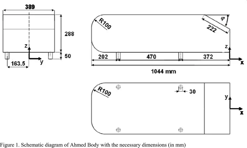
The ground vehicles can be assumed as a bluff body moving in close vicinity of the road surface. The shape of these vehicles has evolved over time keeping in mind various aspects like aesthetics, operational safety, accessibility, etc. But with growing concern over the future availability of fuel as well as the impact of emissions from the vehicles on the environment the improved fuel economy becomes an important requirement for modern vehicles. One of the factors that influence the fuel economy is the drag force that acts on the vehicles as a result of the vehicle shape. So to study this Ahmed et. al. [1] developed an experimental model which is considered as a standard model to understand the flow field structures for the flow around a vehicle.

Due to the simplicity of Ahmed body, as compared to the actual vehicle, it is less costly computationally as well as gives faster results to get an initial idea of the flow field structures.

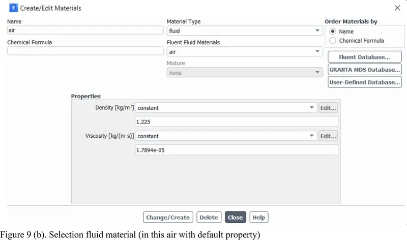
For this problem, air is considered as the fluid with its default properties,

`rho = 1.225 (kg)/m^3`

`mu=1.7894xx10^-5(N.s)/m^2`

As the inlet velocity considered in this challenge is 25 m/s, so the flow can be considered as incompressible as a result there will not be a significant change in the temperature in the flow field. So the fluid properties can be assumed to be constant. 

For Reynolds number calculation overall length of the model (`l=1.044 m`) is considered as the characteristic length. 

Therefore, `Re = (rhoVl)/mu`

`=>Re = (1.225xx25xx1.044)/(1.7894xx10^-5)=1.786xx10^6`

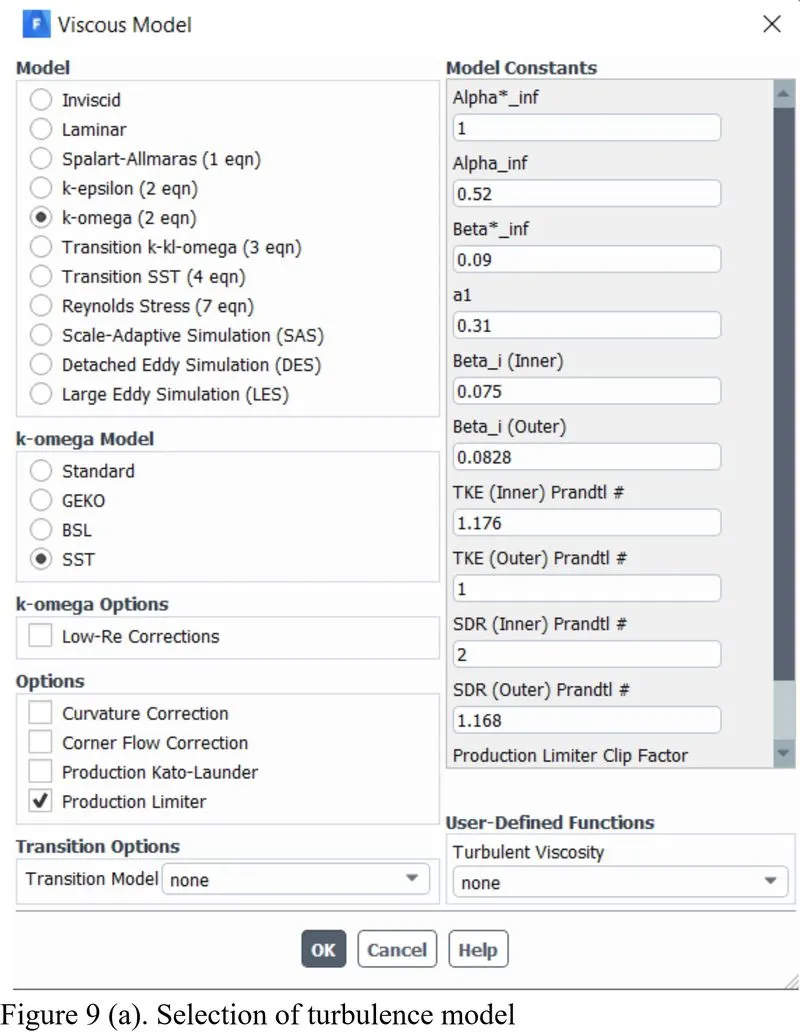
As the inlet flow is turbulent, so to solve this problem `k-omega` SST turbulence model is used. Also, there is a presence of flow separation and reattachment region which is resolved in a better way by this turbulence model.

Model Preparation:

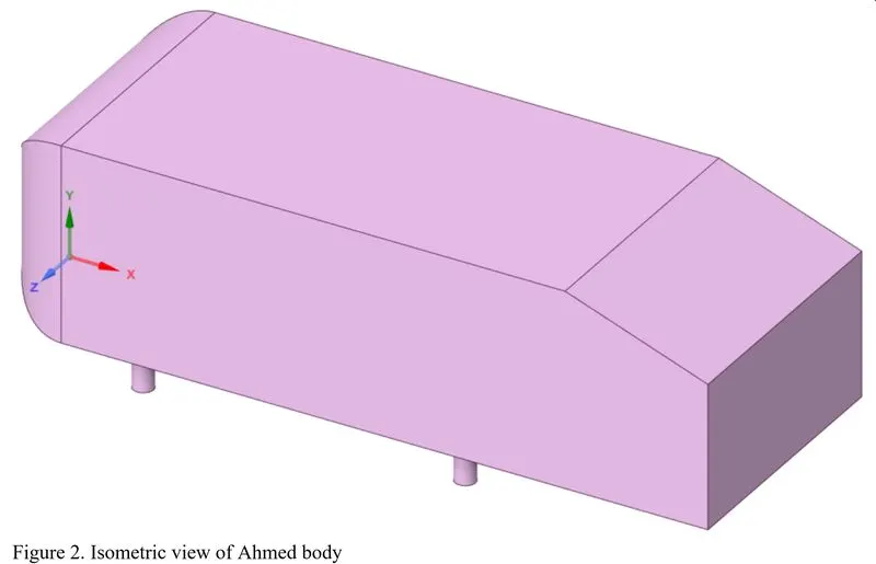
Figure 2 shows the isometric view of the Ahmed body, as this body is symmetric about the X-Y plane so it is wise to cut this body into halves that will reduce the computational time significantly. 

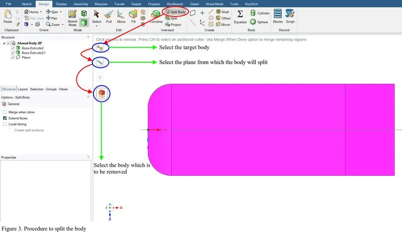
To cut the body, create an X-Y plane and then use the "SPLIT BODY" command as shown in fig. 3

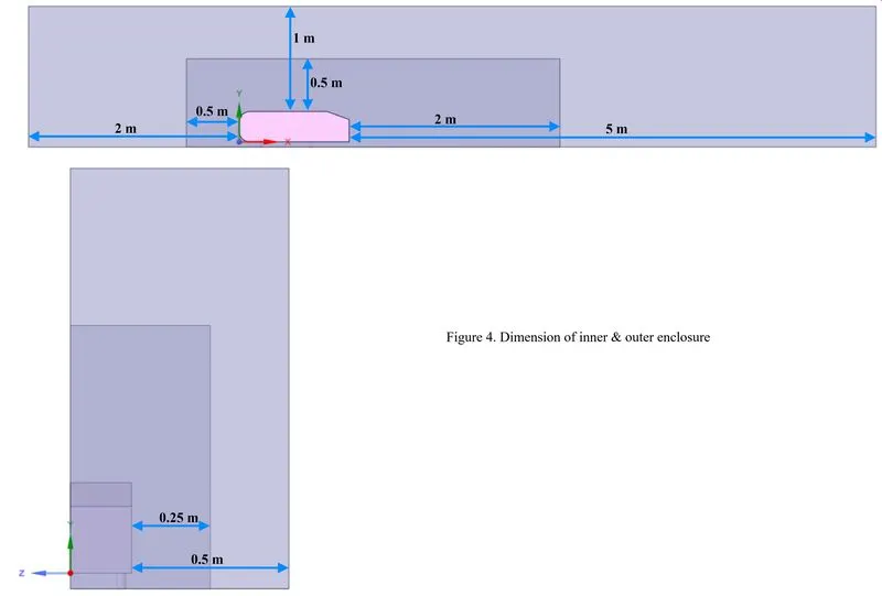
 Once the geometry is split, then the computational domain needs to be created around this. One obvious method to create the computational domain is by drawing the plane one by one enclosing the body but it is time taking. So another easy method is by using the "ENCLOSURE" command. Figure 4 shows the dimension of the inner & outer enclosure. There is a need for two enclosures because to resolve the fluctuation near the Ahmed body we need refined mesh.

Now before proceeding further two important checks is very important because in this challenge two enclosure are being used as to create the computational domain.

1. Check for interference:

This check is necessary to remove the overlap portion of the two enclosures otherwise the mesh in these enclosures will overlap.

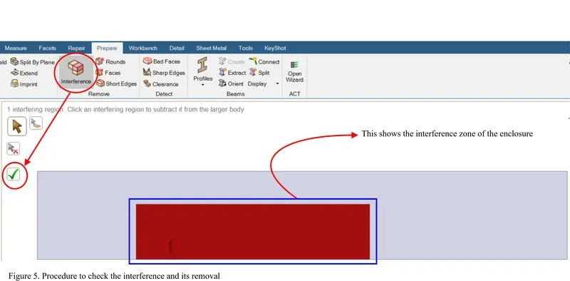
2. Share Topology

As there is 2 enclosure so it should make sure that they share the information across the boundary efficiently for which this procedure is being performed, it is shown in figure 6.

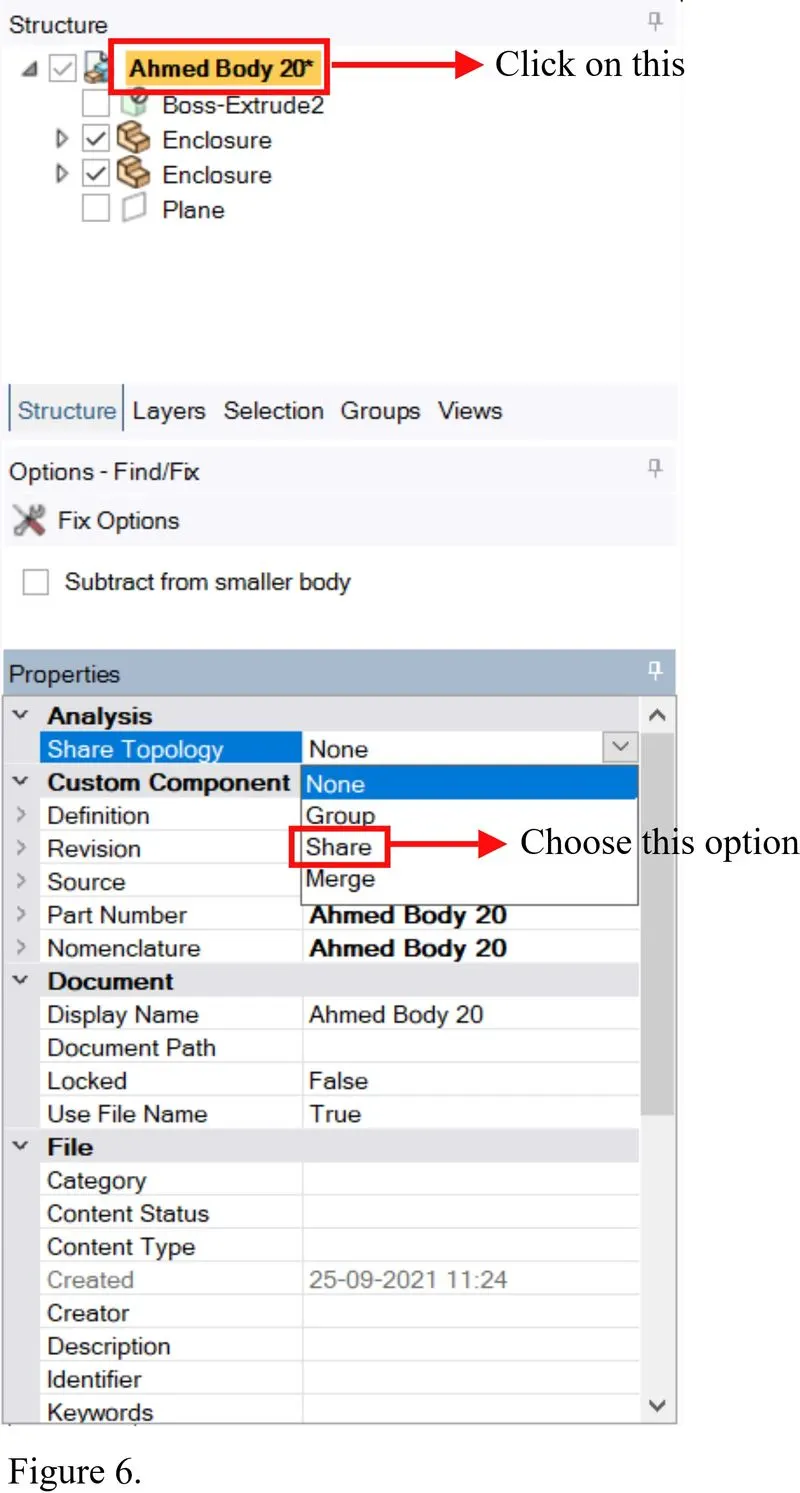
Mesh Generation:

As in this challenge, we have two enclosures and the outer enclosure is made up of a simple straight curve so ideally there should be hexahedral mesh should be used but it is not possible to create the same mesh in the inner enclosure because of the presence of Ahmed body. This is possible by using the "Automatic Method" of mesh generation by choosing the "MultiZone" inside it. The same is shown in figure 7.

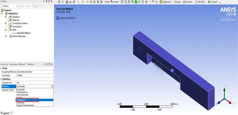
The mesh generated as a result of the above method is shown in figure 8 (a).

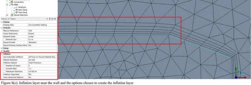
But when we closely observe (fig. 8(b)) the mesh near the wall of the Ahmed body, it can be seen that the grid points are not parallel to the wall as a result the solver will not be able to resolve the flow field variable correctly in the boundary layer region. So for this inflation layer is being added near the wall boundary (fig 8(c)). Ideally, to add the inflation layer the first layer thickness should be equal to y+. For this challenge total thickness is taken as 50 mm consisting of 6 inflation layers with a growth rate of 1.2.

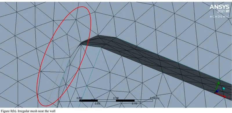
Flow set-up:

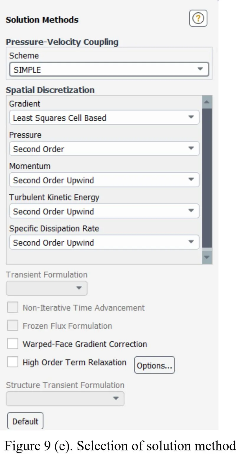
To solve the problem steady-state and pressure-based solver is being used because the velocity at the inlet is 25 m/s which means the Mach number is less than 0.3, so the flow can be assumed to be incompressible. In order to set up the flow physics following procedure is being followed as shown in fig. 9(a) to 9(e).

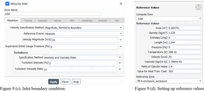
NOTE: References values must be changed like the area which is the frontal area (projected area of the front cross-section) and the length which is the characteristics length, in this case, it is the overall length of the model. This is required to calculate the value of the coefficient of drag and lift accurately.

Results:

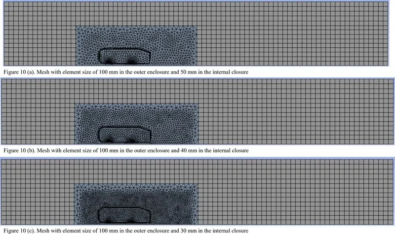
The simulation is performed considering 3 grid size as shown in figure 10 (a), (b), and (c)

 

Velocity Contour:

The velocity contour obtained for all the grid is shown in fig. 11 (a) to (c).

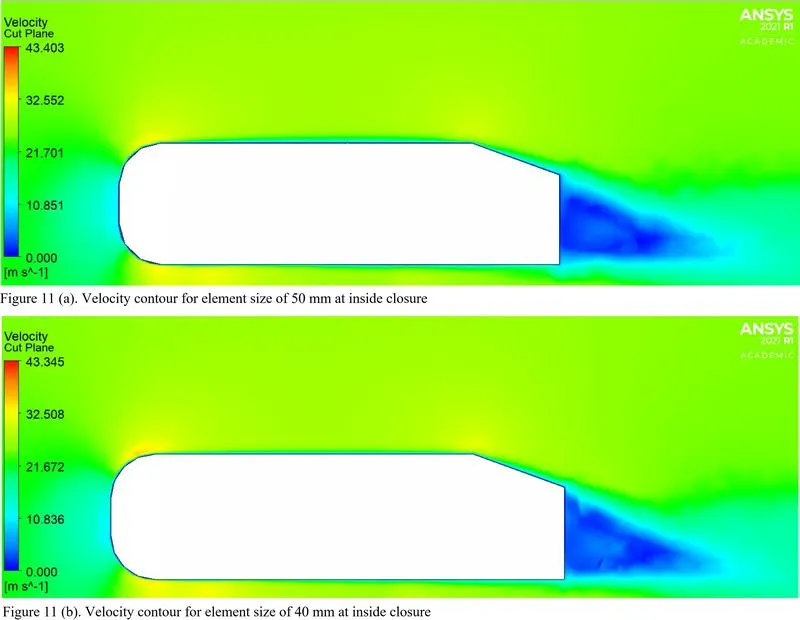
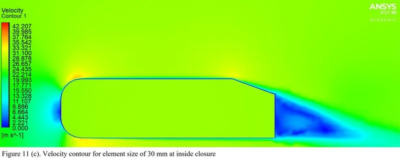
It can be observed that as the grid is refined the resolving capability is improved. 

Velocity Streamline plot:

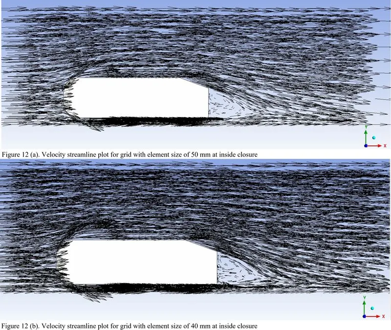
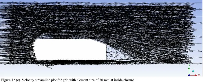
This plot is obtained to observe the recirculation region in the wake zone as shown in fig 12 (a) to (c).

Pressure Contour:

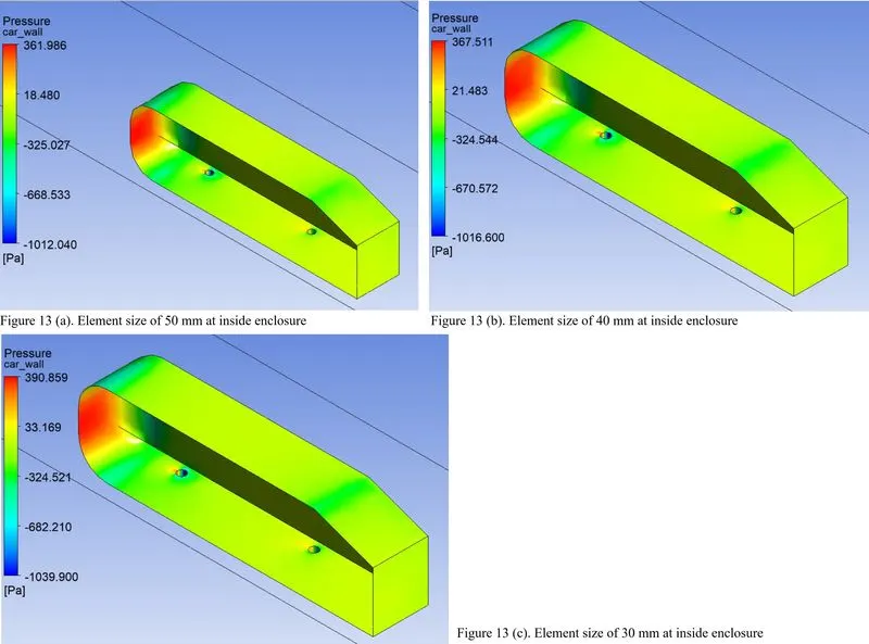
In pressure contours, it can be seen that negative pressure is build up near the top face at the front that is due to the flow separation as the incoming flow faces the bluff body and after some distance, it again reattaches that is due to the momentum transfer from the fluid layer present above it. The flow separation near the top face at the front can also be observed from the streamline plot, fig. 12 (c), where the density of the streamline suddenly reduces.

The coefficient of drag and lift is also computed for every case and is tabulated in table 1.

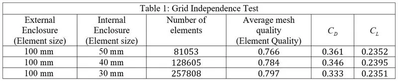
Therefore as the grid is refined the average quality has improved and the same is reflected in the value of the coefficient of drag. 

Conclusion:

1. The coefficient of drag for the given configuration of Ahmed's body (Rear slant angle = `21.8^o`) is 0.33. 

Reference:

1. Some salient features of the time-averaged ground vehicle wake, S.R.Ahmed, G.Ramm & G.Faltin, SAE International, pp. 473-503, 1984.