Week 3 - Adiabatic Flame Temperature calculation
1.Adiabatic flame temperature variation with Equivalence ratio (In constant volume-chamber):
Assume that methane is contained in a constant volume chamber. Write a program in Python to plot the effect of equivalence ratio on the final adiabatic flame temperature.
Calculate the results with Cantera for varying equivalence ratios using the equilibrate method. Assume that N2 is present. Note: There are different parameters present in the equilibrate method. Use correct parameters according to type of combustion.
Compare the results of AFT (at different equivalence ratio) for python and cantera by plotting in a single graph. Explain why AFT of both differs ?
Aim:
To calculate adiabatic flame temperature for different equivalence ratio by writing code in python and by using cantera (equilibrate command). And to plot the results and explain for the variation.
Description:
In this exercise, we will calculate the Adiabatic Flame Temperature for the combustion of methane-air mixture at constant volume and different equivalence ratio by considering ideal products (Stoichiometric products) and by considering equilibrium products (considering dissociation). We will vary the equivalence ratio within the flammability limits of methane-air (0.6-1.4). And then we will compare the AFT results from both the methods.
Procedure:
Python Code for plotting
"""
In this program we are going to calculate the AFT of methaneat differert equivalence ratios
phiCH4 + 2(O2 + N2) = CO2 + 2H2O 7.52N2
"""
import cantera as ct
import numpy as np
import matplotlib.pyplot as plt
import math
T_ad_ideal = []
T_ad_real = []


phi = np.linspace(0.6,1.4,50)
for i in range(0,50):
	# Using ideal products
	# phiCH4 + 2(O2 + N2) = CO2 + 2H2O 7.52N2
	def h(T,co_effs):

		"""
		Function to evaluate enthalpy
		"""
		R = 8.314 #J/Kg-K
		a1 = co_effs[0]
		a2 = co_effs[1]
		a3 = co_effs[2]
		a4 = co_effs[3]
		a5 = co_effs[4]
		a6 = co_effs[5]
		a7 = co_effs[6]
		return (a1 + a2*T/2 + a3*pow(T,2)/3 + a4*pow(T,3)/4 + a5*pow(T,4)/5 + a6/T)*R*T

	CH4_coeffs_l = [5.14987613E+00,-1.36709788E-02, 4.91800599E-05,-4.84743026E-08, 1.66693956E-11,-1.02466476E+04,-4.64130376E+00]
	O2_coeffs_l = [ 3.78245636E+00,-2.99673416E-03, 9.84730201E-06,-9.68129509E-09, 3.24372837E-12,-1.06394356E+03, 3.65767573E+00]
	N2_coeffs_l = [0.03298677E+02, 0.14082404E-02,-0.03963222E-04,0.05641515E-07,-0.02444854E-10,-0.10208999E+04, 0.03950372E+02 ]
	N2_coeffs_h = [0.02926640E+02, 0.14879768E-02,-0.05684760E-05, 0.10097038E-09,-0.06753351E-13,-0.09227977E+04, 0.05980528E+02]
	H2O_coeffs_h = [3.03399249E+00, 2.17691804E-03,-1.64072518E-07,-9.70419870E-11, 1.68200992E-14,-3.00042971E+04, 4.96677010E+00 ]
	CO2_coeffs_h = [3.85746029E+00, 4.41437026E-03,-2.21481404E-06, 5.23490188E-10,-4.72084164E-14,-4.87591660E+04, 2.27163806E+00 ]
	CH4_coeffs_h = [7.48514950E-02, 1.33909467E-02,-5.73285809E-06, 1.22292535E-09,-1.01815230E-13,-9.46834459E+03, 1.84373180E+01]
	O2_coeffs_h = [3.28253784E+00, 1.48308754E-03,-7.57966669E-07, 2.09470555E-10,-2.16717794E-14,-1.08845772E+03, 5.45323129E+00]

	def f(T):
		"""
		function that represents the root finding problem
		"""
		R = 8.314 #J/Kg-K
		if phi[i] == 1:
			H_products = h(T,CO2_coeffs_h) + 2*h(T,H2O_coeffs_h) + 7.52*h(T,N2_coeffs_h)
			n = 10.52
		if phi[i] > 1:
			H_products = h(T,CO2_coeffs_h) + 2*h(T,H2O_coeffs_h) + 7.52*h(T,N2_coeffs_h) + (phi[i]-1)*h(T,CH4_coeffs_h)
			n = 9.52 + phi[i]
		if phi[i] < 1:
			H_products = phi[i]*h(T,CO2_coeffs_h) + 2*phi[i]*h(T,H2O_coeffs_h) + 7.52*h(T,N2_coeffs_h) + 2*(1-phi[i])*h(T,O2_coeffs_h)
			n = 9.52 + phi[i]
		#print(H_products)
		Tstd = 298.15
		H_reactants = phi[i]*h(Tstd,CH4_coeffs_l) + 2*h(Tstd,O2_coeffs_l) + 7.52*h(Tstd,N2_coeffs_l)
		#print(H_reactants)

		return(H_reactants - H_products + n*R*T - (9.52 + phi[i])*R*Tstd)

	def f_prime(T):
		return (f(T+1e-6)-f(T))/1e-6

	T_guess = 1500
	tol = 1e-3
	ct = 0
	alpha = 0.2

	while (abs(f(T_guess)) > tol):
		T_guess = T_guess - alpha*(f(T_guess)/f_prime(T_guess))
		ct =ct+1
	T_ad_ideal.append(T_guess)


	# Using equilibrium composition products
	import cantera as ct
	gas=ct.Solution('gri30.xml')
	gas.TPX = 298.15,101325,{'CH4':phi[i],'O2':2,'N2': 7.52}
	gas.equilibrate('UV',"auto")
	T_ad_real.append(gas.T)


plt.xlabel('Equivalence ratio')
plt.ylabel('Adiabatic Flame Temperature')
plt.grid('on')
plt.plot(phi,T_ad_ideal,'.',color = 'red')
plt.plot(phi,T_ad_real,'.',color = 'blue')
plt.legend(["Ideal products","Real products"])
plt.show()
Results:
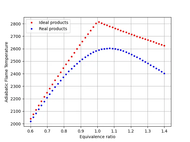
Comments:
From the graph, we can see that for any value of equivalence ratio, ideal products are having more Adiabatic flame temperature. This depends on how the energy is distributed among energy of formation and sensible heat. If the products have less energy of formation and small value of specific heat, then products temperature would be high. The difference in the values of the Adiabatic flame temperature in both cases is because we didnot consider dissociation of products in ideal product case. Since our composition is not accurate, the Adiabatic temperature calculated by that composition is also not accurate.
2. Flame temperature variation with Heat loss (In constant pressure-chamber) :
Consider a constant pressure reactor with heat loss. The reactor is initially set at STP conditions.
The maximum heat loss for the reaction is given below. You will vary the heat loss term by multiplying the “maximum heat loss” with a factor known as H_loss_factor. Example, H_loss_factor = 0.5 would mean a heat loss for that reaction that is equal to 50% of the maximum possible heat loss.
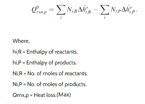
By varying the H_loss_factor from 0 to 1. Plot variation in Flame temperature w.r.t H_loss_factor.
Air:
To find variation of flame temperature with heat loss for stoichiometric composition of methane and air.
Code:
"""
In this program we are going to calculate the FT of methane at stoichiometric composition
CH4 + 2(O2 + N2) = CO2 + 2H2O + 7.52N2
"""
import cantera as ct
import numpy as np
import matplotlib.pyplot as plt
import math
T_flame = []


# Using ideal products
# CH4 + 2(O2 + N2) = CO2 + 2H2O + 7.52N2
def h(T,co_effs):

	"""
	Function to evaluate enthalpy
	"""
	R = 8.314 #J/Kg-K
	a1 = co_effs[0]
	a2 = co_effs[1]
	a3 = co_effs[2]
	a4 = co_effs[3]
	a5 = co_effs[4]
	a6 = co_effs[5]
	a7 = co_effs[6]
	return (a1 + a2*T/2 + a3*pow(T,2)/3 + a4*pow(T,3)/4 + a5*pow(T,4)/5 + a6/T)*R*T

CH4_coeffs_l = [5.14987613E+00,-1.36709788E-02, 4.91800599E-05,-4.84743026E-08, 1.66693956E-11,-1.02466476E+04,-4.64130376E+00]
O2_coeffs_l = [ 3.78245636E+00,-2.99673416E-03, 9.84730201E-06,-9.68129509E-09, 3.24372837E-12,-1.06394356E+03, 3.65767573E+00]
N2_coeffs_l = [0.03298677E+02, 0.14082404E-02,-0.03963222E-04,0.05641515E-07,-0.02444854E-10,-0.10208999E+04, 0.03950372E+02 ]
N2_coeffs_h = [0.02926640E+02, 0.14879768E-02,-0.05684760E-05, 0.10097038E-09,-0.06753351E-13,-0.09227977E+04, 0.05980528E+02]
H2O_coeffs_h = [3.03399249E+00, 2.17691804E-03,-1.64072518E-07,-9.70419870E-11, 1.68200992E-14,-3.00042971E+04, 4.96677010E+00 ]
CO2_coeffs_h = [3.85746029E+00, 4.41437026E-03,-2.21481404E-06, 5.23490188E-10,-4.72084164E-14,-4.87591660E+04, 2.27163806E+00 ]
CO2_coeffs_l = [2.35677352E+00, 8.98459677E-03,-7.12356269E-06, 2.45919022E-09,-1.43699548E-13,-4.83719697E+04, 9.90105222E+00]
H2O_coeffs_l = [4.19864056E+00,-2.03643410E-03 ,6.52040211E-06 ,-5.48797062E-09, 1.77197817E-12,-3.02937267E+04,-8.49032208E-01]

def f(T):
	"""
	function that represents the root finding problem
	"""
	R = 8.314 #J/Kg-K
	if T_guess >= 1000:
		H_products = h(T,CO2_coeffs_h) + 2*h(T,H2O_coeffs_h) + 7.52*h(T,N2_coeffs_h)
	if T_guess < 1000:
		H_products = h(T,CO2_coeffs_l) + 2*h(T,H2O_coeffs_l) + 7.52*h(T,N2_coeffs_l)
	Tstd = 298.15
	H_reactants = h(Tstd,CH4_coeffs_l) + 2*h(Tstd,O2_coeffs_l) + 7.52*h(Tstd,N2_coeffs_l)


	return(H_reactants - H_products - hl[i]*Q_max)

def f_prime(T):
	return (f(T+1e-6)-f(T))/1e-6

#calculating maximum heat loss
hl = [0]
Q_max = 0
T_guess = 200
i = 0
Q_max = abs(f(298.15))

hl =  np.linspace(0,1,100)
for i in range(0,100):

	T_guess = 1500
	tol = 1e-3
	ct = 0
	alpha = 0.2

	while (abs(f(T_guess)) > tol):
		T_guess = T_guess - alpha*(f(T_guess)/f_prime(T_guess))
		ct =ct+1
	T_flame.append(T_guess)


plt.xlabel('Heat loss factor')
plt.ylabel(' Flame Temperature')
plt.title("Flame Temperature vs Heat loss Factor")
plt.grid('on')
plt.plot(hl,T_flame,'.',color = 'red')
plt.show()
Results:
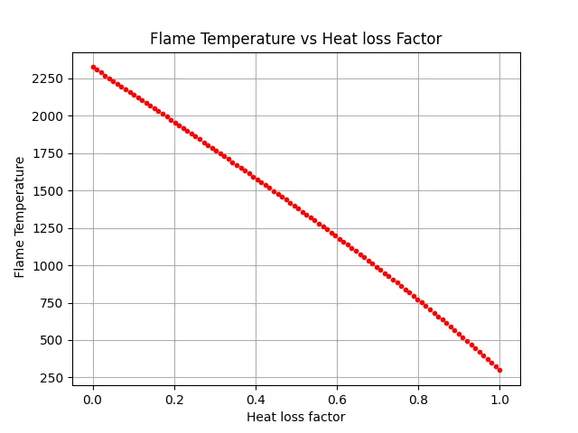
Comments:
Flame temperature decreases as heat is lost from the system.
3. Adiabatic flame temperature variation with respect to Alkane, Alkene, Alkyne :
Test it only for Alk -ane, -ene and -yne variants of 2 Carbon atom chains and plot a trend Assume no heat loss.
Note: Use python coding logic as cantera requires reaction mechanism file and ‘gri30.xml’ file is specifically for methane as fuel.
Aim:
To find the variation of Adiabatic Flame Temperature for the ethane, ethene and ethylene.
Description:
We will find the adiabatic flame temperature for the stoichiometric composition.
Balanced stoichiometric chemical reaction are as follows:
`C_xH_y + ar*(O_2 + 3.76 N_2)->xCO_2 + y/2H_2O + 3.76*arN_2`
where `ar = x+y/4`
Code:
"""
In this program we are going to calculate the AFT at stoichimetric composition
CxHy + ar(O2 + 3.76N2) = xCO2 + y/2H2O + ar*3.76N2
ar = x + y/4
"""
import matplotlib.pyplot as plt
import math
def h(T,co_effs):
	"""
	Function to evaluate enthalpy
	"""
	R = 8.314 #J/Kg-K
	a1 = co_effs[0]
	a2 = co_effs[1]
	a3 = co_effs[2]
	a4 = co_effs[3]
	a5 = co_effs[4]
	a6 = co_effs[5]
	a7 = co_effs[6]
	return (a1 + a2*T/2 + a3*pow(T,2)/3 + a4*pow(T,3)/4 + a5*pow(T,4)/5 + a6/T)*R*T

CH4_coeffs_l = [5.14987613E+00,-1.36709788E-02, 4.91800599E-05,-4.84743026E-08, 1.66693956E-11,-1.02466476E+04,-4.64130376E+00]
C2H6_coeffs_l = [4.29142492E+00,-5.50154270E-03, 5.99438288E-05,-7.08466285E-08, 2.68685771E-11,-1.15222055E+04, 2.66682316E+00]
C3H8_coeffs_l = [0.93355381E+00, 0.26424579E-01, 0.61059727E-05,-0.21977499E-07, 0.95149253E-11,-0.13958520E+05, 0.19201691E+02]
C2H4_coeffs_l = [3.95920148E+00,-7.57052247E-03, 5.70990292E-05,-6.91588753E-08 ,2.69884373E-11, 5.08977593E+03, 4.09733096E+00]
C2H2_coeffs_l = [8.08681094E-01, 2.33615629E-02,-3.55171815E-05,2.80152437E-08,-8.50072974E-12, 2.64289807E+04, 1.39397051E+01]
O2_coeffs_l = [ 3.78245636E+00,-2.99673416E-03, 9.84730201E-06,-9.68129509E-09, 3.24372837E-12,-1.06394356E+03, 3.65767573E+00]
N2_coeffs_l = [0.03298677E+02, 0.14082404E-02,-0.03963222E-04,0.05641515E-07,-0.02444854E-10,-0.10208999E+04, 0.03950372E+02 ]
N2_coeffs_h = [0.02926640E+02, 0.14879768E-02,-0.05684760E-05, 0.10097038E-09,-0.06753351E-13,-0.09227977E+04, 0.05980528E+02]
H2O_coeffs_h = [3.03399249E+00, 2.17691804E-03,-1.64072518E-07,-9.70419870E-11, 1.68200992E-14,-3.00042971E+04, 4.96677010E+00 ]
CO2_coeffs_h = [3.85746029E+00, 4.41437026E-03,-2.21481404E-06, 5.23490188E-10,-4.72084164E-14,-4.87591660E+04, 2.27163806E+00 ]
x = [2,2,2]
y = [6,4,2]
Tad = []
# finding Tad for methane ethane and propane


def f(T):
	"""
	function that represents the root finding problem
	"""
	ar  = x[i] + y[i]/4
	if i == 0:
		H_products = x[i]*h(T,CO2_coeffs_h) + (y[i]/2)*h(T,H2O_coeffs_h) + ar*3.76*h(T,N2_coeffs_h)
		#print(H_products)
		Tstd = 298.15
		H_reactants = h(Tstd,C2H6_coeffs_l) + ar*h(Tstd,O2_coeffs_l) + 3.76*ar*h(Tstd,N2_coeffs_l)
		#print(H_reactants)
		#return(H_reactants - H_products)
	if i == 1:
		H_products = x[i]*h(T,CO2_coeffs_h) + (y[i]/2)*h(T,H2O_coeffs_h) + ar*3.76*h(T,N2_coeffs_h)
		#print(H_products)
		Tstd = 298.15
		H_reactants = h(Tstd,C2H4_coeffs_l) + ar*h(Tstd,O2_coeffs_l) + 3.76*ar*h(Tstd,N2_coeffs_l)
		#print(H_reactants)
		#return(H_reactants - H_products)
	if i == 2:
		H_products = x[i]*h(T,CO2_coeffs_h) + (y[i]/2)*h(T,H2O_coeffs_h) + ar*3.76*h(T,N2_coeffs_h)
		#print(H_products)
		Tstd = 298.15
		H_reactants = h(Tstd,C2H2_coeffs_l) + ar*h(Tstd,O2_coeffs_l) + 3.76*ar*h(Tstd,N2_coeffs_l)
		#print(H_reactants)
	return(H_reactants - H_products)

def f_prime(T):
	return (f(T+1e-5)-f(T))/1e-5


tol = 1e-4
alpha = 0.2
for i in range(0,3):
	T_guess = 3000
	ct = 0
	while (abs(f(T_guess)) > tol):
		T_guess = T_guess - alpha*(f(T_guess)/f_prime(T_guess))
		#plt.plot(ct,T_guess,'*',color = 'red')
		print(T_guess)
		ct =ct+1
	Tad.append(T_guess)

print(Tad)
data = {'C2H6':Tad[0],'C2H4':Tad[1],'C2H2':Tad[2]}

#fig = plt.figure(figsize = (10, 5))

# creating the bar plot
plt.bar(list(data.keys()), list(data.values()), color ='blue',width = 0.4)

plt.xlabel("Fuel")
plt.ylabel("Adiabatic Flame Temperature")
plt.title("Adiabatic Flame Temperature vs fuel")
plt.show()
Results:
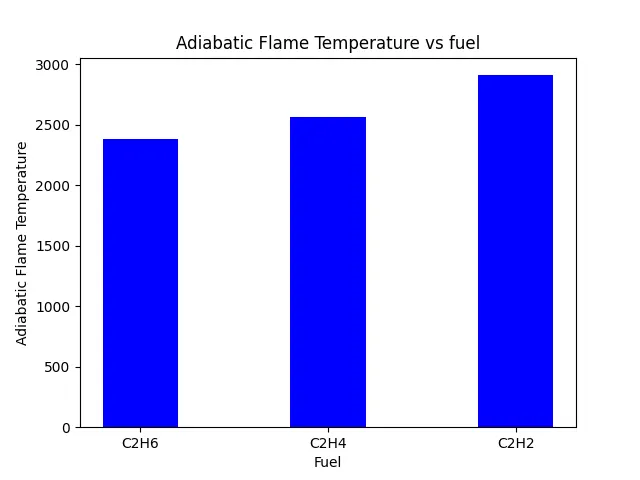

Comments:
Adiabatic temperature increases with decrease in number of hydrogen atoms. This is because upon combustion, hydrogen is converted to water vapour and it takes more heat for energy of formation and sensible energy.
4. Adiabatic flame temperature variation with respect to number of Carbon atom chains :
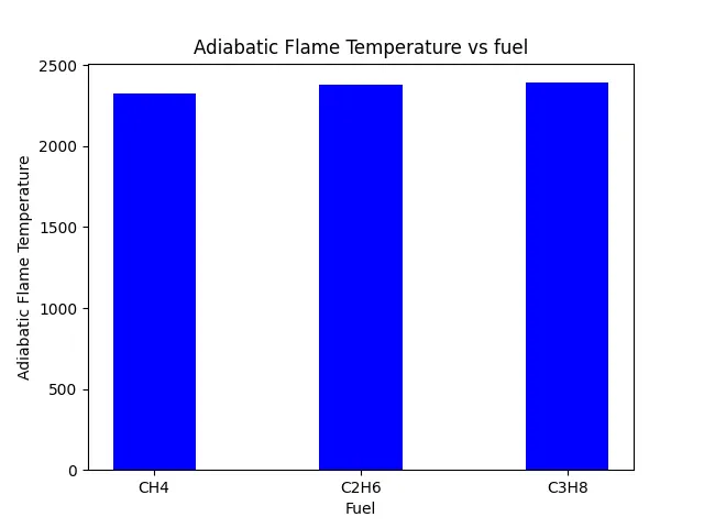
For a general alkane, plot the effect of the number of carbon atoms (from 1 to 3) on the final temperature. Assume no heat loss.
Note: Use python coding logic as cantera requires reaction mechanism file and ‘gri30.xml’ file is specifically for methane as fuel.
Aim:
To find the effect of Adiabatic Flame Temperature variation with respect to number of carbon atoms in alkanes.
Description:
We will find the adiabatic flame temperature for the stoichiometric composition for methane ethane and propane..
Balanced stoichiometric chemical reaction are as follows:
`C_xH_y + ar*(O_2 + 3.76 N_2)->xCO_2 + y/2H_2O + 3.76*arN_2`
where `ar = x+y/4`
Code:
"""
In this program we are going to calculate the AFT at stoichimetric composition
CxHy + ar(O2 + 3.76N2) = xCO2 + y/2H2O + ar*3.76N2
ar = x + y/4
"""
import matplotlib.pyplot as plt
import math
def h(T,co_effs):
	"""
	Function to evaluate enthalpy
	"""
	R = 8.314 #J/Kg-K
	a1 = co_effs[0]
	a2 = co_effs[1]
	a3 = co_effs[2]
	a4 = co_effs[3]
	a5 = co_effs[4]
	a6 = co_effs[5]
	a7 = co_effs[6]
	return (a1 + a2*T/2 + a3*pow(T,2)/3 + a4*pow(T,3)/4 + a5*pow(T,4)/5 + a6/T)*R*T

CH4_coeffs_l = [5.14987613E+00,-1.36709788E-02, 4.91800599E-05,-4.84743026E-08, 1.66693956E-11,-1.02466476E+04,-4.64130376E+00]
C2H6_coeffs_l = [4.29142492E+00,-5.50154270E-03, 5.99438288E-05,-7.08466285E-08, 2.68685771E-11,-1.15222055E+04, 2.66682316E+00]
C3H8_coeffs_l = [0.93355381E+00, 0.26424579E-01, 0.61059727E-05,-0.21977499E-07, 0.95149253E-11,-0.13958520E+05, 0.19201691E+02]
C2H4_coeffs_l = [3.95920148E+00,-7.57052247E-03, 5.70990292E-05,-6.91588753E-08 ,2.69884373E-11, 5.08977593E+03, 4.09733096E+00]
C2H2_coeffs_l = [8.08681094E-01, 2.33615629E2,-3.55171815E-05,2.80152437E-08,-8.50072974E-12, 2.64289807E+04, 1.39397051E+01]
O2_coeffs_l = [ 3.78245636E+00,-2.99673416E-03, 9.84730201E-06,-9.68129509E-09, 3.24372837E-12,-1.06394356E+03, 3.65767573E+00]
N2_coeffs_l = [0.03298677E+02, 0.14082404E-02,-0.03963222E-04,0.05641515E-07,-0.02444854E-10,-0.10208999E+04, 0.03950372E+02 ]
N2_coeffs_h = [0.02926640E+02, 0.14879768E-02,-0.05684760E-05, 0.10097038E-09,-0.06753351E-13,-0.09227977E+04, 0.05980528E+02]
H2O_coeffs_h = [3.03399249E+00, 2.17691804E-03,-1.64072518E-07,-9.70419870E-11, 1.68200992E-14,-3.00042971E+04, 4.96677010E+00 ]
CO2_coeffs_h = [3.85746029E+00, 4.41437026E-03,-2.21481404E-06, 5.23490188E-10,-4.72084164E-14,-4.87591660E+04, 2.27163806E+00 ]
x = [1,2,3]
y = [4,6,8]
Tad = []
# finding Tad for methane ethane and propane


def f(T):
	"""
	function that represents the root finding problem
	"""
	ar  = x[i] + y[i]/4
	if i == 0:
		H_products = x[i]*h(T,CO2_coeffs_h) + (y[i]/2)*h(T,H2O_coeffs_h) + ar*3.76*h(T,N2_coeffs_h)
		#print(H_products)
		Tstd = 298.15
		H_reactants = h(Tstd,CH4_coeffs_l) + ar*h(Tstd,O2_coeffs_l) + 3.76*ar*h(Tstd,N2_coeffs_l)
		#print(H_reactants)
		#return(H_reactants - H_products)
	if i == 1:
		H_products = x[i]*h(T,CO2_coeffs_h) + (y[i]/2)*h(T,H2O_coeffs_h) + ar*3.76*h(T,N2_coeffs_h)
		#print(H_products)
		Tstd = 298.15
		H_reactants = h(Tstd,C2H6_coeffs_l) + ar*h(Tstd,O2_coeffs_l) + 3.76*ar*h(Tstd,N2_coeffs_l)
		#print(H_reactants)
		#return(H_reactants - H_products)
	if i == 2:
		H_products = x[i]*h(T,CO2_coeffs_h) + (y[i]/2)*h(T,H2O_coeffs_h) + ar*3.76*h(T,N2_coeffs_h)
		#print(H_products)
		Tstd = 298.15
		H_reactants = h(Tstd,C3H8_coeffs_l) + ar*h(Tstd,O2_coeffs_l) + 3.76*ar*h(Tstd,N2_coeffs_l)
		#print(H_reactants)
	return(H_reactants - H_products)

def f_prime(T):
	return (f(T+1e-5)-f(T))/1e-5


tol = 1e-4
alpha = 0.2
for i in range(0,3):
	T_guess = 3000
	ct = 0
	while (abs(f(T_guess)) > tol):
		T_guess = T_guess - alpha*(f(T_guess)/f_prime(T_guess))
		#plt.plot(ct,T_guess,'*',color = 'red')
		print(T_guess)
		ct =ct+1
	Tad.append(T_guess)

print(Tad)
data = {'CH4':Tad[0],'C2H6':Tad[1],'C3H8':Tad[2]}

#fig = plt.figure(figsize = (10, 5))

# creating the bar plot
plt.bar(list(data.keys()), list(data.values()), color ='blue',width = 0.4)

plt.xlabel("Fuel")
plt.ylabel("Adiabatic Flame Temperature")
plt.title("Adiabatic Flame Temperature vs fuel")
plt.show()
Results:

Comments:
Adiabatic flame temperature is increasing with increase in the number of carbon atoms in the fuel.