Week 3 - Adiabatic Flame Temperature calculation

Objective

To determine the effect of equivalent ratio, carbon content and type of fuel on the Adiabatic Flame Temperature in both constant volume and constant pressure reaction.

Theory

When a combustion reaction takes place energy is released to the combustion products. If no heat is lost in this process, the temperature of the combustion products is known as the Adiabatic Flame Temperature.

In the study of combustion, there are two types of adiabatic flame temperature depending on how the process is completed: the constant volume and constant pressure; both of which describe temperature that combustion products theoretically can reach if no energy is lost to the outside environment.

The constant volume adiabatic flame temperature is the temperature that results from a complete combustion process that occurs without any work, heat transfer or changes in kinetic or potential energy. Its temperature is higher than the constant pressure process because no energy is utilized to change the volume of the system.

For Constant Volume Reaction, the enthalpy of reaction is given as

`H_("reactions") = H_("products") - H_("reactants") - (N_("products") - N_("reactants"))`

while for constant Pressure reaction, it is given as:

`H_("reactions") = H_("products") - H_("reactants")`

Whenever there is Heat loss, however, the enthalpy of reaction for constant pressure reaction is modified as

`H_("reactions") = H_("products") - H_("reactants") + (H_("loss")timesLHV)`

where `H_("loss")` is the factor that expresses the fraction of heat lost.

Present Study

The present study considers Methane combustion in a constant volume. The general equation of reaction is given as:

`CH_4 + a(O_2 + 3.76N_2) => bCO_2 + cH_2O + dO_2 +eCO + f3.76N_2`

And depending on the equivalence ratio,`phi`, some constants are zero

if `phi < 1 =>` lean combustion. e = 0

if `phi = 1 =>` stoichiometric combustion. d = e = 0.

if `phi >1 =>` rich combustion. d = 0.

So a python code was developed to evaluate the effect of `phi` on the adiabatic flame temperature, `T_(AFT)`, for combustion in constant volume. The calulation is iterative in nature and Newton-Raphson method was used here. The same was done using cantera. The codes and the results are displayed below.

import cantera as ct
import numpy as np 
import matplotlib.pyplot as plt
%matplotlib inline 


CH4_coeffs_l = [5.14987613E+00, -1.36709788E-02, 4.91800599E-05, -4.84743026E-08, 1.66693956E-11, -1.02466476E+04, -4.64130376E+00];
O2_coeffs_l = [3.78245636E+00, -2.99673416E-03, 9.84730201E-06, -9.68129509E-09,  3.24372837E-12, -1.06394356E+03,  3.65767573E+00];
O2_coeffs_h = [3.28253784E+00, 1.48308754E-03, -7.57966669E-07, 2.09470555E-10, -2.16717794E-14, -1.08845772E+03, 5.45323129E+00]
N2_coeffs_l = [0.03298677E+02, 0.14082404E-02, -0.03963222E-04, 0.05641515E-07, -0.02444854E-10, -0.10208999E+04, 0.03950372E+02];
N2_coeffs_h = [0.02926640E+02, 0.14879768E-02, -0.05684760E-05, 0.10097038E-09, -0.06753351E-13, -0.09227977E+04, 0.05980528E+02];
H2O_coeffs_h = [3.03399249E+00, 2.17691804E-03, -1.64072518E-07, -9.70419870E-11, 1.68200992E-14, -3.00042971E+04, 4.96677010E+00];
CO2_coeffs_h = [3.85746029E+00, 4.41437026E-03, -2.21481404E-06, 5.23490188E-10, -4.72084164E-14, -4.87591660E+04, 2.27163806E+00];
CO_coeffs_h = [2.71518561E+00, 2.06252743E-03, -9.98825771E-07, 2.30053008E-10, -2.03647716E-14, -1.41518724E+04, 7.81868772E+00];


def enthalpy(T, coeffs):
    R = 8.314;
    a1 = coeffs[0];
    a2 = coeffs[1];
    a3 = coeffs[2];
    a4 = coeffs[3];
    a5 = coeffs[4];
    a6 = coeffs[5];
    return (a1 + a2*T/2 + a3*pow(T,2)/3 + a4*pow(T,3)/4 + a5*pow(T,4)/5 + a6/T)*R*T



def reaction(T_stp, T, phi):
    R = 8.314;
    
    h_r_CH4 = enthalpy(T_stp, CH4_coeffs_l);
    h_r_O2 = enthalpy(T_stp, O2_coeffs_l);
    h_r_N2 = enthalpy(T_stp, N2_coeffs_l);
    
    N_reactants = (1 + (2/phi) + (7.52/phi));
    H_reactants = h_r_CH4 + (2/phi)*h_r_O2 + (7.52/phi)*h_r_N2;
    
    h_p_CO2 = enthalpy(T, CO2_coeffs_h);
    h_p_H2O = enthalpy(T, H2O_coeffs_h);
    h_p_O2 = enthalpy(T, O2_coeffs_h);
    h_p_CO = enthalpy(T, CO_coeffs_h);
    h_p_N2 = enthalpy(T, N2_coeffs_h);
    
    if phi < 1:
        N_products = (1  + 2 + (2/phi-2)  + (7.52/phi));
        H_products = h_p_CO2 + 2*h_p_H2O + (2/phi-2)*h_p_O2 + (7.52/phi)*h_p_N2;
    elif phi >= 1:
        N_products = ((4/phi - 3) + 2 + (4-4/phi) + (7.52/phi));
        H_products = (4/phi - 3)*h_p_CO2 + 2*h_p_H2O + (4-4/phi)*h_p_CO + (7.52/phi)*h_p_N2;
    
    return (H_products - H_reactants) - R*(T*N_products - T_stp*N_reactants)

def reaction_prime(T_stp, T, phi):
    return (reaction(T_stp, T+1e-6, phi) - reaction(T_stp, T, phi))/(1e-6)

T_AFT_calc = [];
alpha = 0.2;
phi = [x/10 for x in range(1,21)];
tol = 1e-3;

for i in range(0, len(phi)):
    T_stp = 298.15;
    T_guess = 1500;
    while (abs(reaction(T_stp, T_guess, phi[i])) >= tol):
        T_guess -= alpha*(reaction(T_stp, T_guess, phi[i])/reaction_prime(T_stp, T_guess, phi[i]));
    T_AFT_calc.append(T_guess);
        


gas1 = ct.Solution('gri30.xml');
T_AFT_ct = [];
for i in range(0, len(phi)):
    T_stp = 298.15;
    P = 101325;
    n_total = 1 + 2/phi[i] + 7.52/phi[i];
    n_CH4 = 1/n_total;
    n_O2 = 2/(phi[i]*n_total);
    n_N2 = 7.52/(phi[i]*n_total);
    gas1.TPX = T_stp, P, {'CH4':n_CH4, 'O2':n_O2, 'N2':n_N2};
    gas1.equilibrate('UV', 'auto');
    T_AFT_ct.append(gas1.T);



plt.plot(phi, T_AFT_calc, 'ks-', color='blue', label='Calculated')
plt.plot(phi, T_AFT_ct, 'ks-', color='black', label='Cantera')
plt.xlabel('Equivalence Ratio, $\phi$', fontsize=12)
plt.ylabel('Adiabatic Flame Temperature, $T_{AFT}$ [K]', fontsize=12)
plt.title('$T_{AFT}$ vs $\phi$ for $CH_4$-$O_2$ Combustion', fontsize=15, fontweight='bold')
plt.legend(fontsize=12)
plt.show()

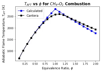
From the plot above, the code developed was not far off from cantera's output.

Next, the effect of heat loss is considered on the flame temperature for stoichiometric combustion in a constant pressure chamber. This was also done using the Newton-Raphson iterative method. The codes and the results are also displayed below

def LHV():
    return enthalpy(T_stp, CH4_coeffs_l) + 2*enthalpy(T_stp, O2_coeffs_l) - enthalpy(T_stp, CO2_coeffs_h) - 2*enthalpy(T_stp, H2O_coeffs_h);


def reaction_with_heat_loss(T, H_loss):
    T_stp = 298.15;
    h_r_CH4 = enthalpy(T_stp, CH4_coeffs_l);
    h_r_O2 = enthalpy(T_stp, O2_coeffs_l);
    h_r_N2 = enthalpy(T_stp, N2_coeffs_l);
    H_reactants = h_r_CH4 + 2*h_r_O2 + 7.52*h_r_N2;
    
    
    h_p_CO2 = enthalpy(T, CO2_coeffs_h);    
    h_p_H2O = enthalpy(T, H2O_coeffs_h);
    h_p_N2 = enthalpy(T, N2_coeffs_h);
    H_products = h_p_CO2 + 2*h_p_H2O + 7.52*h_p_N2;
    
    return H_products - H_reactants + (H_loss*LHV())



def reaction_with_heat_loss_prime(T, H_loss):
    return (reaction_with_heat_loss(T+1e-6, H_loss) - reaction_with_heat_loss(T, H_loss))/1e-6


H_loss = [x/10 for x in range(0, 11)];
tol =1e-3;
T_F_wloss = [];
alpha = 0.2
for i in range(0, len(H_loss)):
    T_guess = 1500;
    while (abs(reaction_with_heat_loss(T_guess, H_loss[i])) >=tol):
        T_guess -= alpha*(reaction_with_heat_loss(T_guess, H_loss[i])/reaction_with_heat_loss_prime(T_guess, H_loss[i]));
    T_F_wloss.append(T_guess);


plt.plot(H_loss, T_F_wloss, 'ks-', color='black')
plt.xlabel('Fractional Heat Loss, $\\theta$', fontsize=12)
plt.ylabel(' Flame Temperature, $T_{Flame}$ [K]', fontsize=12)
plt.title('$T_{Flame}$ vs $\\theta$ for $CH_4$-$O_2$ Combustion', fontsize=15, fontweight='bold')
plt.show()

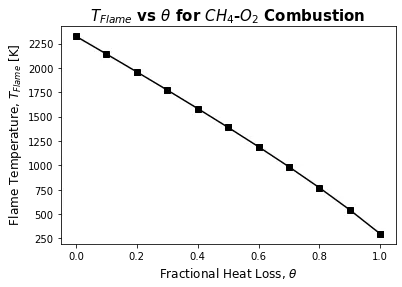
A decreasing trend is observed from the plot above.

Next, the flame temperature for different types of 2-Carbon fuels is considered. These fuels are burned in a constant pressure combustor with heat loss, `H_("loss") = 0.35`. The fuels considered are Ethane (`C_2H_6`), Ethene(`C_2H_4`), and Ethyne(`C_2H_2`). The process is the same as described above.

C2H2_coeffs_l = [8.08681094E-01, 2.33615629E-02, -3.55171815E-05, 2.80152437E-08, -8.50072974E-12, 2.64289807E+04, 1.39397051E+01];
C2H4_coeffs_l = [3.95920148E+00, -7.57052247E-03, 5.70990292E-05, -6.91588753E-08, 2.69884373E-11, 5.08977593E+03, 4.09733096E+00];
C2H6_coeffs_l = [4.29142492E+00, -5.50154270E-03, 5.99438288E-05, -7.08466285E-08, 2.68685771E-11, -1.15222055E+04, 2.66682316E+00];

def LHV_with_var_fuel(n_H):
    n_C = 2;
    
    if n_H == 2:
        h_r_fuel =  enthalpy(T_stp, C2H2_coeffs_l);
    elif n_H == 4:
        h_r_fuel = enthalpy(T_stp, C2H4_coeffs_l);
    elif n_H == 6:
        h_r_fuel =  enthalpy(T_stp, C2H6_coeffs_l);
        
    return h_r_fuel + (n_C + n_H/4)*enthalpy(T_stp, O2_coeffs_l) + 3.76*(n_C + n_H/4)*enthalpy(T_stp, N2_coeffs_l) - n_C*enthalpy(T_stp, CO2_coeffs_h) -  n_H/2*enthalpy(T_stp, H2O_coeffs_h)- 3.76*(n_C + n_H/4)*enthalpy(T_stp, N2_coeffs_h);

def reaction_with_var_fuel(T, n_H):
    T_stp = 298.15;
    H_loss = 0.35;
    n_C = 2;
    
    if n_H == 2:
        h_r_fuel =  enthalpy(T_stp, C2H2_coeffs_l);
    elif n_H == 4:
        h_r_fuel = enthalpy(T_stp, C2H4_coeffs_l);
    elif n_H == 6:
        h_r_fuel =  enthalpy(T_stp, C2H6_coeffs_l);
        
    h_r_O2 = enthalpy(T_stp, O2_coeffs_l);
    h_r_N2 = enthalpy(T_stp, N2_coeffs_l);
    H_reactants = h_r_fuel + (n_C + n_H/4)*h_r_O2 + 3.76*(n_C + n_H/4)*h_r_N2;
    
    
    h_p_CO2 = enthalpy(T, CO2_coeffs_h);    
    h_p_H2O = enthalpy(T, H2O_coeffs_h);
    h_p_N2 = enthalpy(T, N2_coeffs_h);
    H_products = n_C*h_p_CO2 + n_H/2*h_p_H2O + 3.7*(n_C + n_H/4)*h_p_N2;
    
    return H_products - H_reactants + (H_loss*LHV_with_var_fuel(n_H))


def reaction_with_var_fuel_prime(T, n_H):
    return (reaction_with_var_fuel(T+1e-6, n_H) - reaction_with_var_fuel(T, n_H))/1e-6

n_H = [6, 4, 2];
tol =1e-3;
T_F_vfuel = [];
alpha = 0.2
for i in range(0, len(n_H)):
    T_guess = 1500;
    while (abs(reaction_with_var_fuel(T_guess, n_H[i])) >=tol):
        T_guess -= alpha*(reaction_with_var_fuel(T_guess,n_H[i])/reaction_with_var_fuel_prime(T_guess, n_H[i]));
    T_F_vfuel.append(T_guess);


fig = plt.figure()
ax = fig.add_axes([0,0,1,1])
fuels = ['Ethane', 'Ethene', 'Ethyne']
ax.bar(fuels,T_F_vfuel, color='black')
plt.xlabel('Two-Carbon Fuels', fontsize=12)
plt.ylabel('Flame Temperature, $T_{Flame}$ [K]', fontsize=12)
plt.title('$T_{Flame}$ for Two-Carbon fuels Combustion', fontsize=15, fontweight='bold')
plt.show()

Ethyne is found to have the highest flame temperature. This is due to the triple bonds between the carbon atoms in the fuel chemical structure. Breaking all three requires the highest amount of heat compared to the rest.

Next, the effect of the number of carbon atoms in a fuel chemical structure on Adiabatic Flame Temperature was considered. For this, the first three members of the alkane family of fuels was use. They are Methane(`CH_4`), Ethane (`C_2H_6`), and Propane(`C_2H_8`).

C3H8_coeffs_l = [0.93355381E+00, 0.26424579E-01, 0.61059727E-05, -0.21977499E-07, 0.95149253E-11, -0.13958520E+05, 0.19201691E+02];



def alkane_reaction(T, n_C):
    n_H = 2*n_C+2;
    T_stp = 298.15;
    if n_C == 1:
        h_r_fuel = enthalpy(T_stp, CH4_coeffs_l);
    elif n_C == 2:
        h_r_fuel = enthalpy(T_stp, C2H6_coeffs_l);
    elif n_C == 3:
        h_r_fuel = enthalpy(T_stp, C3H8_coeffs_l);
        
    h_r_O2 = enthalpy(T_stp, O2_coeffs_l);
    h_r_N2 = enthalpy(T_stp, N2_coeffs_l);
    H_reactants = h_r_fuel + (n_C + n_H/4)*h_r_O2 + 3.76*(n_C + n_H/4)*h_r_N2;
    
    h_p_CO2 = enthalpy(T, CO2_coeffs_h);    
    h_p_H2O = enthalpy(T, H2O_coeffs_h);
    h_p_N2 = enthalpy(T, N2_coeffs_h);
    
    H_products = n_C*h_p_CO2 +  n_H/2*h_p_H2O + 3.76*(n_C + n_H/4)*h_p_N2;    
    
    return H_products - H_reactants



def alkane_reaction_prime(T, n_C):
    return (alkane_reaction(T+1e-06, n_C) - alkane_reaction(T, n_C))/1e-06



n_C = [1, 2, 3];
alkanes = ['Methane', 'Ethane', 'Propane'];
tol =1e-3;
T_AFT_alkanes = [];
alpha = 0.2
for i in range(0, len(n_C)):
    T_guess = 1500;
    while (abs(alkane_reaction(T_guess, n_C[i])) >=tol):
        T_guess -= alpha*(alkane_reaction(T_guess,n_C[i])/alkane_reaction_prime(T_guess, n_C[i]));
    T_AFT_alkanes.append(T_guess);
    


fig = plt.figure()
ax = fig.add_axes([0,0,1,1])
ax.bar(alkanes,T_AFT_alkanes, color='green')
plt.xlabel('Alkane Fuels', fontsize=12)
plt.ylabel('Adiabatic Flame Temperature, $T_{AFT}$ [K]', fontsize=12)
plt.title('$T_{AFT}$ for Alkane fuels Combustion', fontsize=15, fontweight='bold')
plt.show()

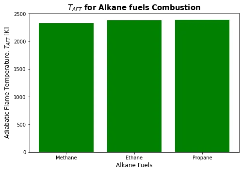
Propane has a slightly highest `T_(AFT)`. However, it is not enough to favour it above other alkane fuels. Other factors such as perhaps, it's density would hav to be considered.