Week 9 - FVM Literature Review
Objective
This project is about review of essentials of Finite Volume Method, especially to,
- understand what Finite Volume Method (FVM) is
- understand the major differences between FDM & FVM
- understand the need for interpolation schemes and flux limiters in FVM
What is Finite Volume Method (FVM)
The finite volume method (FVM) is a method for representing and evaluating partial differential equations in the form of algebraic equations. In the finite volume method, volume integrals in a partial differential equation that contain a divergence term are converted to surface integrals, using the divergence theorem. These terms are then evaluated as fluxes at the surfaces of each finite volume. Because the flux entering a given volume is identical to that leaving the adjacent volume, these methods are conservative.
Another advantage of the finite volume method is that it is easily formulated to allow for unstructured meshes. The method is used in many computational fluid dynamics packages. "Finite volume" refers to the small volume surrounding each node point on a mesh.
Differences between FDM & FVM
| FDM | FVM |
|
FDM is a differential scheme, that is approximation of a taylor series expansion. the first order, second order differentials are written in terms of difference between two point values. This may bring in some approximation error. |
Finite Volume method is an integral scheme. Since integration is across the area, chance of error is minimized. |
|
FDM schemes are faster and error can be minimized for regular grids such as squares and rectangles |
FVM schemes are slightly slower but can be faster than FDM when the mesh is irregular. |
Interpolation Schemes
The approximations to the integrals require the values of variables at locations other than computational nodes (CV centers). To calculate the convective and diffusive fluxes, the value of and its gradient normal to the cell face at one or more locations on the CV surface are needed. Volume integrals of the source terms may also require these values. They have to be expressed in terms of the nodal values by interpolation.
Numerous interpolation schemes are available. The most commonly used ones are mentioned below.
Upwind interpolation scheme (UDS)
This is also called Upwind differencing Scheme (UDS) and the `phi_e` is approximated as:

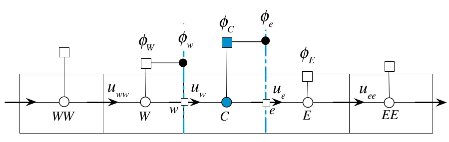
UDS is
- first-order accurate
- unconditionally stable(i.e. no oscillations)
- numerically diffusive
Linear Interpolation (CDS)
Another straightforward approximation for the value at CV-face center is linear interpolation between the two nearest nodes. At location 'e' on a Cartesian grid we have
`phi_e = lambda_e phi_E + (1 - lambda_e) phi_P`
`lambda_e = (x_e - x_P)/(x_E - x_P)`
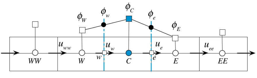
CDS is
- second-order accurate
- the simplest second-order scheme and is widely used
- may produce oscillatory solutions
Quadratic Upwind Interpolation (QUICK)
QUICK, which stands for Quadratic Upstream Interpolation for Convective Kinematics, is a higher-order differencing scheme that considers a three-point upstream weighted quadratic interpolation for the cell face values. For the one dimensional convection-diffusion problem under discussion, the value of `phi` is computed using
`phi = k_0 + k_1x + k_2x^2`
subject to,
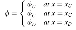
Applying the conditions given, the profile for `phi` is found to be

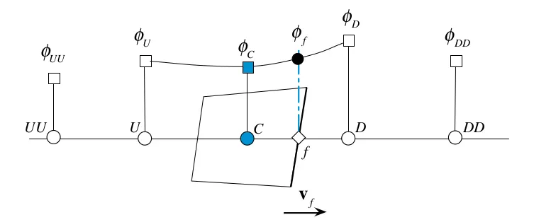
QUICK scheme
- is more complex than CDS
- has third-order truncation error
- is second-order accurate when used in conjunction with the midpoint-rule approximation of the surface integral.
Flux Limiters
Flux limiters are used in high resolution schemes such as the MUSCL Schemes to avoid the spurious oscillations (wiggles) that would otherwise occur with high order spatial discretization schemes due to shocks, discontinuities or sharp changes in the solution domain. Use of flux limiters, together with an appropriate high resolution scheme, make the solutions Total variation Diminishing (TVD).
Flux limiters are also referred to as slope limiters because they both have the same mathematical form, and both have the effect of limiting the solution gradient near shocks or discontinuities.
In general, the term flux limiter is used when the limiter acts on system fluxes, and slope limiter is used when the limiter acts on system states (like pressure, velocity etc.).
The main idea behind the construction of flux limiter schemes is to limit the spatial derivatives to realistic values – for scientific and engineering problems this usually means physically realisable and meaningful values. So, they only come into operation when sharp wave fronts are present. For smoothly changing waves, the flux limiters do not operate and the spatial derivatives can be represented by higher order approximations without introducing spurious oscillations.
Consider the 1D semi-discrete scheme below,
`(du)/(dt) + 1/(Delta x_i) [F(u_(i+1/2) )+ F(u_(i-1/2))] = 0`
where `F(u_(i+1/2) )+ F(u_(i-1/2))` are the edge fluxes for the ith cell. Representing these edge fluxes by low and high resolution schemes means a flux limiter can switch between these schemes depending upon the gradients close to the particular cell. This is depicted as follows


 `"low resolution flux"`
 `"high resolution flux"`
 `"flux limiter function"`
and `r` represents the ratio of successive gradients on the solution mesh, i.e.,

The limiter function is constrained to be greater than or equal to zero, i.e. `phi(r) ge 0`. Therefore, when the limiter is equal to zero (sharp gradient, opposite slopes or zero gradient), the flux is represented by a low resolution scheme. Similarly, when `phi(r) = 1` (smooth solution), it is represented by a high resolution scheme.
The various limiters have differing switching characteristics and are selected according to the particular problem and solution scheme.
No particular limiter has been found to work well for all problems, and a particular choice is usually made on a trial and error basis.