Week 11 - Simulation of Flow through a pipe in OpenFoam

Objective

This project studies simulation of incompressible flow in a circular pipe using a piece of the geometry. Specifically, it aims to

• understand how the wedge angle influences accuracy of results
• understand the flow phenomenon and compare to available analytic results
• compare the flow velocity and shear stress distribution against Hagen-Poiseuille's equation

Theory

The study of fluid dynamics is divided into two types:

• External fluid flow
• Internal fluid flow

Internal flow is a flow for which the fluid is confined by a surface. Hence the boundary layer is unable to develop without eventually being constrained. The internal flow configuration represents a convenient geometry for heating and cooling fluids used in chemical processing, environmental control, and energy conversion technologies.

For internal fluid flow, one of the representative cases is the incompressible laminar flow through a circular pipe. This is the Hagen-Poiseuille flow.

In non-ideal fluid dynamics, the Hagen–Poiseuille law, also known as the Hagen–Poiseuille equation, Poiseuille law or Poiseuille equation, is a physical law that gives the pressure drop in an incompressible and Newtonian fluid in laminar flow flowing through a long cylindrical pipe of constant cross section. The assumptions of the equation are that the fluid is incompressible and Newtonian; the flow is laminar through a pipe of constant circular cross-section that is substantially longer than its diameter; and there is no acceleration of fluid in the pipe.

The Hagen–Poiseuille equation can be derived from the Navier–Stokes equations in 3D cylindrical co-ordinates. The laminar flow through a pipe of uniform (circular) cross-section is known as Hagen–Poiseuille flow.

`1/rdel/(delr)(r(delu)/(delr)) = 1/mu (dp)/(dx)`

`u = -(DeltaP r^2)/(4muL) + c_1lnr +c_2`

and with conditions,

`r =0, u=infty => c_1=0`

`r = R, u=0 => c_2 = (DeltaP R^2)/(4muL)`

so that the velocity profile becomes,

` u = (DeltaP)/(4muL)(R^2 - r^2)`

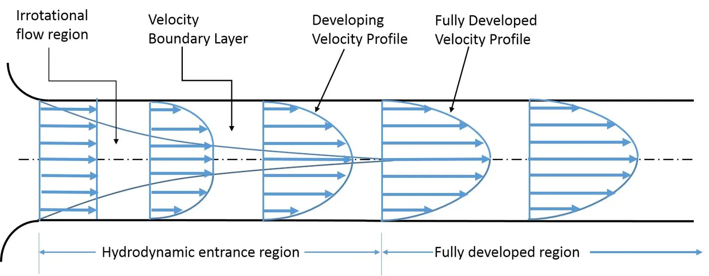
However, for internal flow like in a circular pipe, the flow is not fully developed throughout the whole pipe length. It has to travel a distance before it becomes fully developed. This distance is called entrance length.

Entrance length refers to the length of the entry region, the area following the pipe entrance where effects originating from the interior wall of the pipe propagate into the flow as an expanding boundary layer. When the boundary layer expands to fill the entire pipe, the developing flow becomes a fully developed flow, where flow characteristics no longer change with increased distance along the pipe. Many different entrance lengths exist to describe a variety of flow conditions. Hydrodynamic entrance length describes the formation of a velocity profile caused by viscous forces propagating from the pipe wall.

The length of the hydrodynamic entry region along the pipe is called the hydrodynamic entry length. It is a function of Reynolds number of the flow. In case of laminar flow, this length is given by:

`L_(h,laminar) approx 0.06R_eD`

And for the flow to remain laminar. the flow Reynolds number, `Re approx 2300`.

Flow Variables

For the present study, the working fluid is oil with following parameters:

• `rho = 900 kg"/"m^3`
• `mu = 0.0288 Pa.s`

The pipe dimensions are

• `D = 10 mm`
• `R_e = 150`
• `L_h = 0.06 times 150 times 1 = 9mm`
• `L_("pipe") = L_h + 150 = 159mm`

The flow parameters are thus derived below:

• `u_"avg" = (mu R_e)/(rho D) = 0.48 m"/"s`
• `u_"max" =2times u_"avg" = 0.96m"/"s`
• `DeltaP = (32mu L u_"avg")/D^2 = 703.365 Pa`
• `P_"kinematic" = (DeltaP)/rho = 0.7815m`
• `tau(r) = (2mu u_"max"R)/r^2 = (2.7648 times 10^-4)/r^2 Pa`

Numerical Simulation

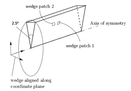
Numerical simulations were carried for a wedge of the cylindrical domain. The angle of the wedge was varied in order to observe its impact on the accuracy of solutions.

An octave script was written to generate the blockMeshDict file. The script calls modular functions that generates different sections of the file from the OpenFoam Header to the Boundary section. These are displayed belowed.

function foamHeader(objectName, conversion)
  foamHead = fopen('blockMeshDict', 'w');
  fprintf(foamHead, '%s\n', '/*--------------------------------*- C++ -*----------------------------------*\');
  fprintf(foamHead, '%s\n', '  =========                 |');
  fprintf(foamHead, '%s\n', '  \\      /  F ield         | OpenFOAM: The Open Source CFD Toolbox');
  fprintf(foamHead, '%s\n', '   \\    /   O peration     | Website:  https://openfoam.org');
  fprintf(foamHead, '%s\n', '    \\  /    A nd           | Version:  7');
  fprintf(foamHead, '%s\n', '     \\/     M anipulation  |');
  fprintf(foamHead, '%s\n', '\*---------------------------------------------------------------------------*/');
  fprintf(foamHead, '%s\n', 'FoamFile');
  fprintf(foamHead, '%s\n', '{');
  fprintf(foamHead, '%s\n', '    version     2.0;');
  fprintf(foamHead, '%s\n', '    format      ascii;');
  fprintf(foamHead, '%s\n', '    class       dictionary;');
  fprintf(foamHead, '%s %s %s\n', '    object     ', objectName, ';');
  fprintf(foamHead, '%s\n', '}');
  fprintf(foamHead, '%s\n\n', '// * * * * * * * * * * * * * * * * * * * * * * * * * * * * * * * * * * * * * //');
  fprintf(foamHead, '%s %d %s\n\n', 'convertToMeters ', conversion, ';');
  fclose(foamHead);
 end

function foamVertices(diameter, theta, length)
   radius = diameter/2;
   foamVertex = fopen('blockMeshDict', 'a');
   fprintf(foamVertex, '%s\n', 'vertices');
   fprintf(foamVertex, '%s\n', '(');
   fprintf(foamVertex, '%s\n', '    (0 0 0)              //0');
   fprintf(foamVertex, '%s %f %f %s\n', '    (0', radius*cosd(theta/2), -radius*sind(theta/2),')              //1');
   fprintf(foamVertex, '%s %f %f %s\n', '    (0', radius*cosd(theta/2), radius*sind(theta/2),')              //2');
   fprintf(foamVertex, '%s%f %s\n', '    (',length, ' 0 0)              //3');
   fprintf(foamVertex, '%s%f %f %f%s\n', '    (',length, radius*cosd(theta/2), -radius*sind(theta/2),')              //4');
   fprintf(foamVertex, '%s%f %f %f%s\n', '    (',length, radius*cosd(theta/2), radius*sind(theta/2),')              //5');
   fprintf(foamVertex, '%s\n\n', ');');
   
   fclose(foamVertex);
   end

function foamBlocks(grids, gradings);
  foamBlock = fopen('blockMeshDict', 'a');
  fprintf(foamBlock, '%s\n', 'blocks');
  fprintf(foamBlock, '%s\n', '(');
  fprintf(foamBlock, '%s %s %s %s \n', '    hex (0 1 2 0 3 4 5 3)', grids, 'simpleGrading', gradings);
  fprintf(foamBlock, '%s\n\n', ');');
  
  fclose(foamBlock);
 end

function foamEdges(edge_1, edge_2);
  foamEdge = fopen('blockMeshDict', 'a');
  fprintf(foamEdge, '%s\n', 'edges');
  fprintf(foamEdge, '%s\n', '(');
  fprintf(foamEdge, '%s %s\n', '    arc 1 2', edge_1);
  fprintf(foamEdge, '%s %s\n', '    arc 4 5', edge_2);
  fprintf(foamEdge, '%s\n\n', ');');
  
  fclose(foamEdge);
 end

function foamBoundaries(b_names, b_types, b_faces)
  foamBoundary = fopen('blockMeshDict', 'a');
  fprintf(foamBoundary, '%s\n', 'boundary');
  fprintf(foamBoundary, '%s\n', '(');
  for i = 1:length(b_names)
    fprintf(foamBoundary, '%s%s\n', '    ', b_names{i,1});
    fprintf(foamBoundary, '%s\n', '    {');
    fprintf(foamBoundary, '%s %s%s\n', '        type', b_types{i,1}, ';');
    fprintf(foamBoundary, '%s\n', '        faces');
    fprintf(foamBoundary, '%s\n', '        (');
    fprintf(foamBoundary, '%s%s\n', '            ', b_faces{i,1});
    fprintf(foamBoundary, '%s\n', '        );');
    fprintf(foamBoundary, '%s\n', '    }');
  end
  fprintf(foamBoundary, '%s\n\n', ');');
  fprintf(foamBoundary, '%s\n', 'mergePatchPairs');
  fprintf(foamBoundary, '%s\n', '(');
  fprintf(foamBoundary, '%s\n\n', ');');
  
  fprintf(foamBoundary, '%s\n', '// ************************************************************************* //');
  
  fclose(foamBoundary)
end

clear all; close all; clc;

%inputs
diameter = 10; %mm
theta = 4; %degrees
length = 159; %mm

grids = '(50 1 100)';
gradings = '(0.1 1 10)';

edge_1 = '(0 5 0)';
edge_2 = '(159 5 0)';

b_names = {"inlet"; "outlet"; "wall"; "axis"; "front"; "back"};
b_faces = {"(1 0 0 2)"; "(5 3 3 4)"; "(2 5 4 1)"; "(0 3 3 0)"; "(0 3 5 2)"; "(0 1 4 3)"};
b_types = {"patch"; "patch"; "wall"; "empty"; "wedge"; "wedge"};

foamHeader('blockMeshDict', 0.001);
foamVertices(diameter, theta, length);
foamBlocks(grids, gradings);
foamEdges(edge_1, edge_2);
foamBoundaries(b_names, b_types, b_faces);

The output of the script is displayed below

/*--------------------------------*- C++ -*----------------------------------*\
  =========                 |
  \\      /  F ield         | OpenFOAM: The Open Source CFD Toolbox
   \\    /   O peration     | Website:  https://openfoam.org
    \\  /    A nd           | Version:  7
     \\/     M anipulation  |
\*---------------------------------------------------------------------------*/
FoamFile
{
    version     2.0;
    format      ascii;
    class       dictionary;
    object      blockMeshDict ;
}
// * * * * * * * * * * * * * * * * * * * * * * * * * * * * * * * * * * * * * //

convertToMeters  0.001 ;

vertices
(
    (0 0 0)              //0
    (0 4.996954 -0.174497 )              //1
    (0 4.996954 0.174497 )              //2
    (159.000000  0 0)              //3
    (159.000000 4.996954 -0.174497)              //4
    (159.000000 4.996954 0.174497)              //5
);

blocks
(
    hex (0 1 2 0 3 4 5 3) (50 1 100) simpleGrading (0.1 1 10) 
);

edges
(
    arc 1 2 (0 5 0)
    arc 4 5 (159 5 0)
);

boundary
(
    inlet
    {
        type patch;
        faces
        (
            (1 0 0 2)
        );
    }
    outlet
    {
        type patch;
        faces
        (
            (5 3 3 4)
        );
    }
    wall
    {
        type wall;
        faces
        (
            (2 5 4 1)
        );
    }
    axis
    {
        type empty;
        faces
        (
            (0 3 3 0)
        );
    }
    front
    {
        type wedge;
        faces
        (
            (0 3 5 2)
        );
    }
    back
    {
        type wedge;
        faces
        (
            (0 1 4 3)
        );
    }
);

mergePatchPairs
(
);

// ************************************************************************* //

OpenFOAM cases were setup for wedge angles, `theta = 2, 3, 4, `. The initial conditions and controlDict files are displayed for case `theta=5`. The remaining cases are similar except for the `theta`-value. For the time step, from the CFL condition,

`C = Delta t [u/(Delta x) + w/(Delta z)] le 0.5`

`=> Delta t le (CDelta x)/u`

because `w = 0` at initial condition.

/*--------------------------------*- C++ -*----------------------------------*\
  =========                 |
  \\      /  F ield         | OpenFOAM: The Open Source CFD Toolbox
   \\    /   O peration     | Website:  https://openfoam.org
    \\  /    A nd           | Version:  7
     \\/     M anipulation  |
\*---------------------------------------------------------------------------*/
FoamFile
{
    version     2.0;
    format      ascii;
    class       volScalarField;
    object      p;
}
// * * * * * * * * * * * * * * * * * * * * * * * * * * * * * * * * * * * * * //

dimensions      [0 2 -2 0 0 0 0];

internalField   uniform 0;

boundaryField
{
    inlet
    {
        type            zeroGradient;
    }

    outlet
    {
        type            fixedValue;
        value           uniform 0.7815;
    }

    wall
    {
        type            zeroGradient;
    }
    
    axis
    {
        type            empty;
    }
 
    front
    {
        type            wedge;
    }

    back
    {
        type            wedge;
    }
}

// ************************************************************************* //

/*--------------------------------*- C++ -*----------------------------------*\
  =========                 |
  \\      /  F ield         | OpenFOAM: The Open Source CFD Toolbox
   \\    /   O peration     | Website:  https://openfoam.org
    \\  /    A nd           | Version:  7
     \\/     M anipulation  |
\*---------------------------------------------------------------------------*/
FoamFile
{
    version     2.0;
    format      ascii;
    class       volVectorField;
    object      U;
}
// * * * * * * * * * * * * * * * * * * * * * * * * * * * * * * * * * * * * * //

dimensions      [0 1 -1 0 0 0 0];

internalField   uniform (0.48 0 0);

boundaryField
{
    inlet
    {
        type            fixedValue;
        value           uniform (0.48 0 0);
    }

    outlet
    {
        type            inletOutlet;
        inletValue      uniform (0.48 0 0);
        value           uniform (0.48 0 0);
    }

    wall
    {
        type            fixedValue;
        value           uniform (0 0 0);
    }
    
    axis
    {
        type            empty;
    }
 
    front
    {
        type            wedge;
    }

    back
    {
        type            wedge;
    }
}

// ************************************************************************* //

/*--------------------------------*- C++ -*----------------------------------*\
  =========                 |
  \\      /  F ield         | OpenFOAM: The Open Source CFD Toolbox
   \\    /   O peration     | Website:  https://openfoam.org
    \\  /    A nd           | Version:  7
     \\/     M anipulation  |
\*---------------------------------------------------------------------------*/
FoamFile
{
    version     2.0;
    format      ascii;
    class       dictionary;
    location    "system";
    object      controlDict;
}
// * * * * * * * * * * * * * * * * * * * * * * * * * * * * * * * * * * * * * //

application     icoFoam;

startFrom       startTime;

startTime       0;

stopAt          endTime;

endTime         0.2;

deltaT          0.00005;

writeControl    timeStep;

writeInterval   20;

purgeWrite      0;

writeFormat     ascii;

writePrecision  6;

writeCompression off;

timeFormat      general;

timePrecision   6;

runTimeModifiable true;


// ************************************************************************* //

Results and Analysis

Wedge angle =2

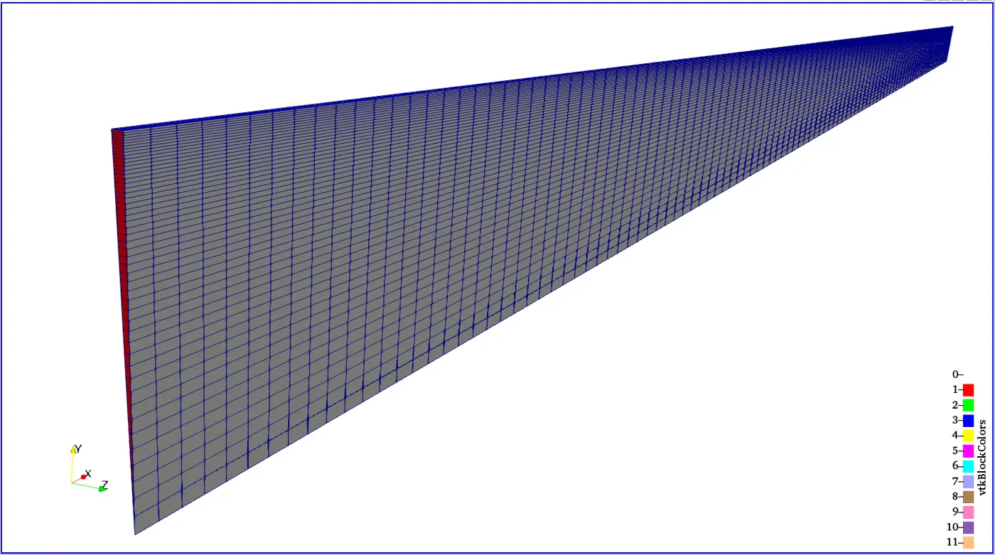
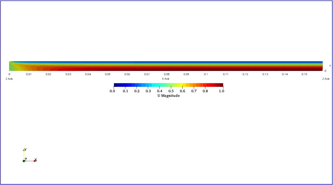
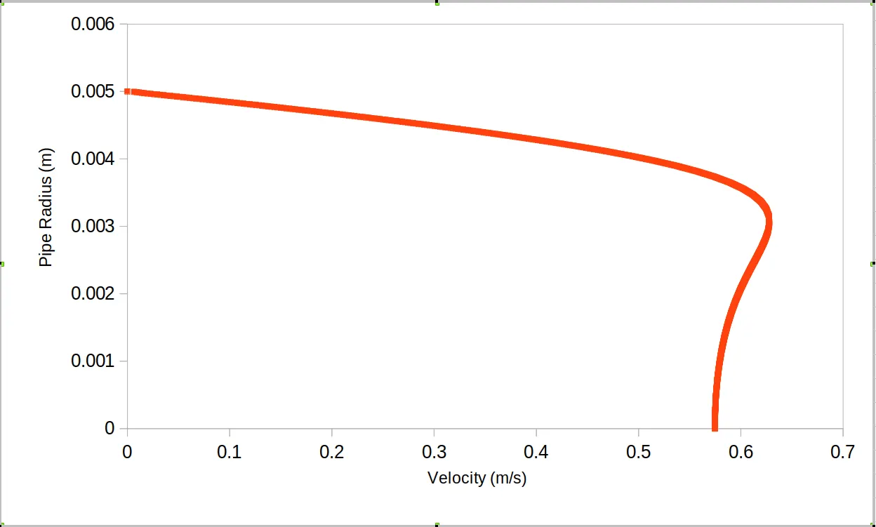
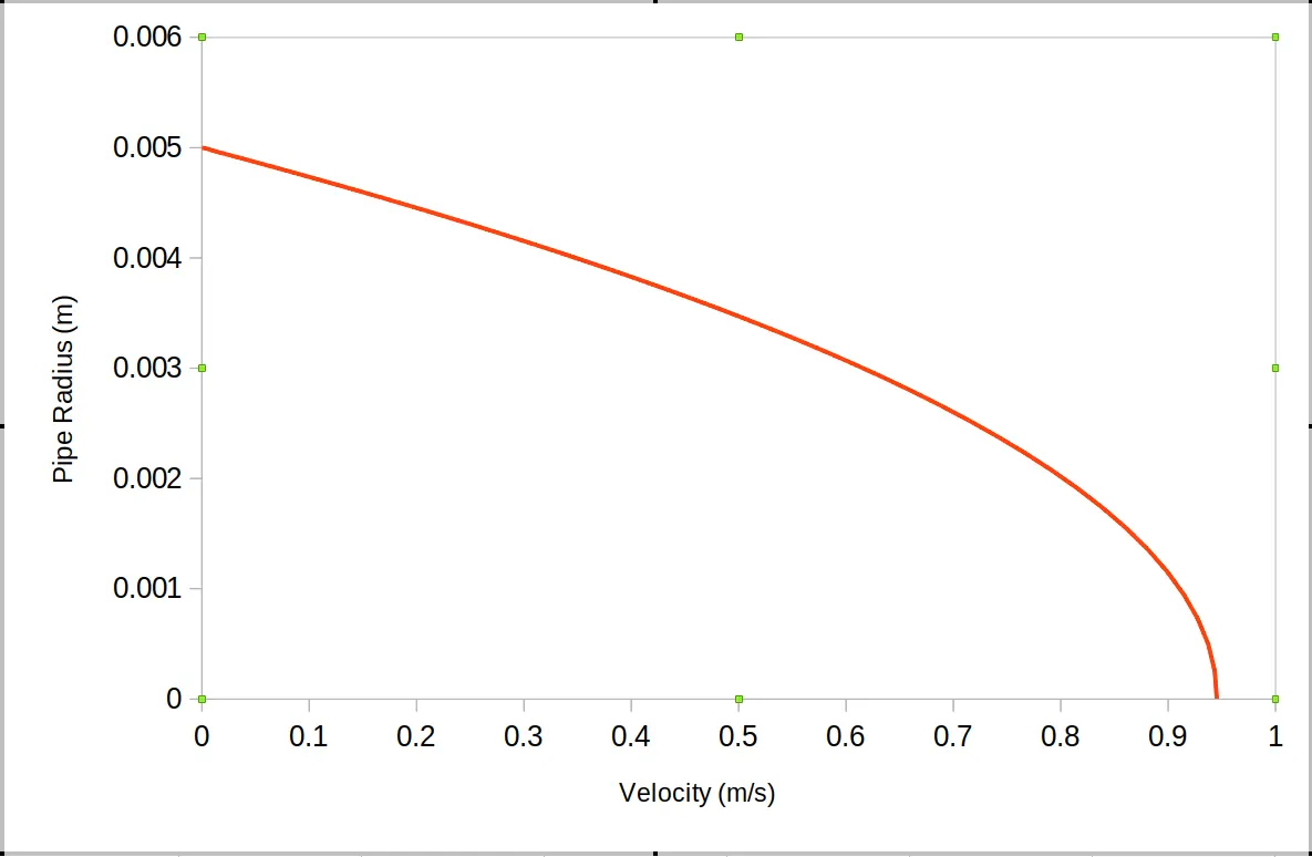
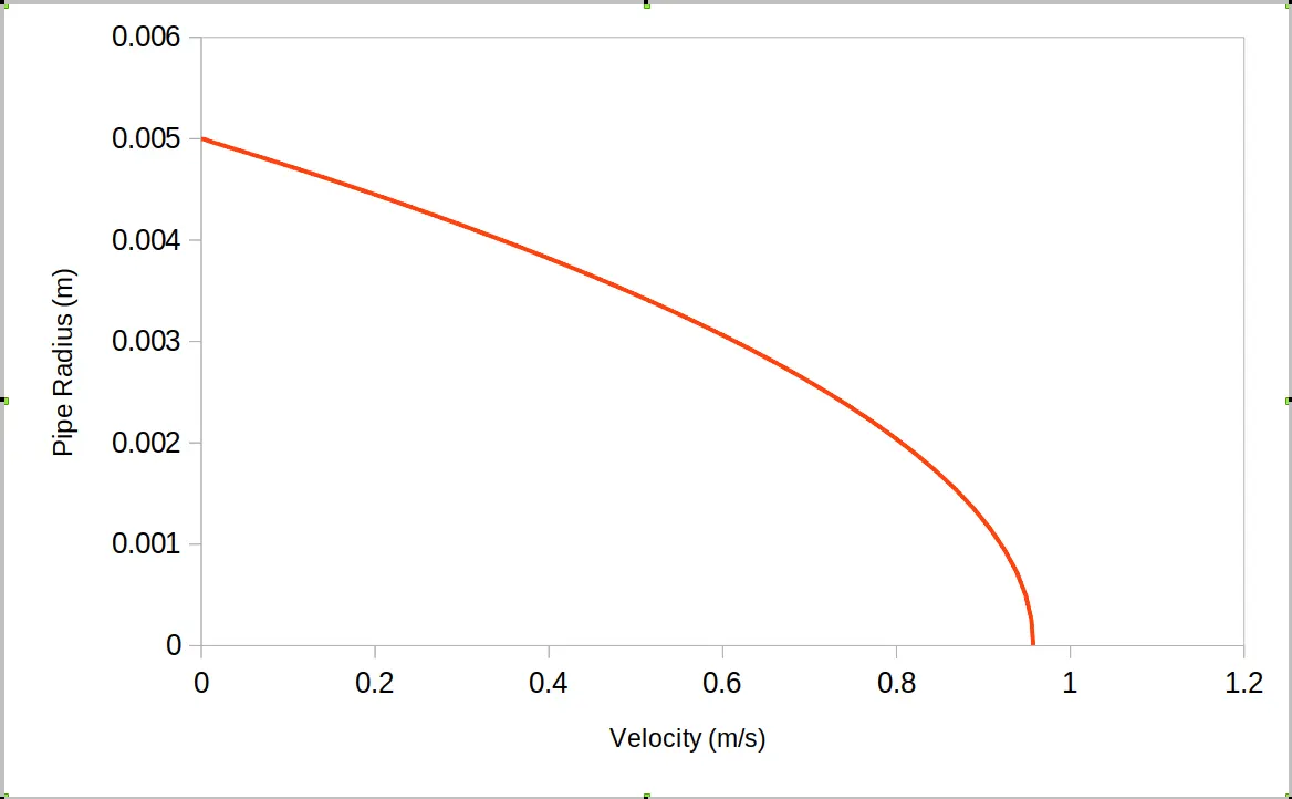
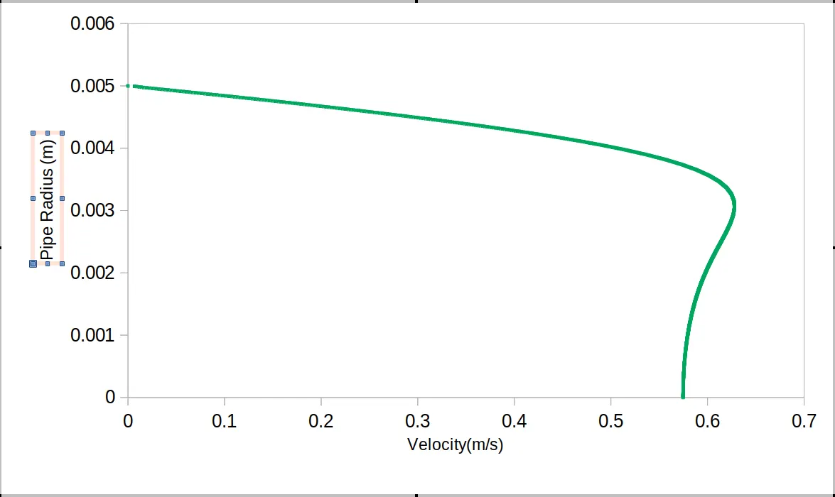
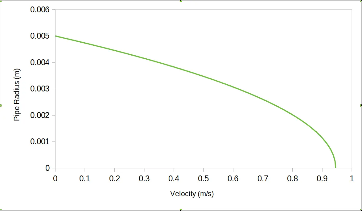
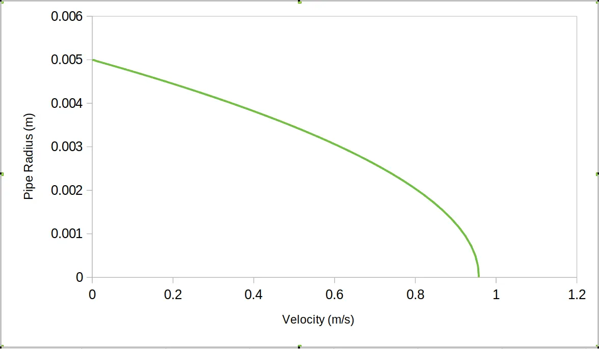
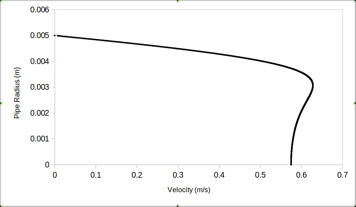
The mesh generated for the domains are displayed below for `theta = 2`. The result of the velocity distrbution inside the pipe is also displayed. The velocity profile at various planes in the x-axis (`x =0.005, 0.0795, 0.155`) were also plotted. The first plane is within the developing region(` x = 0 - 0.009`) while the remaining two in the fully developed region with one close to the exit.

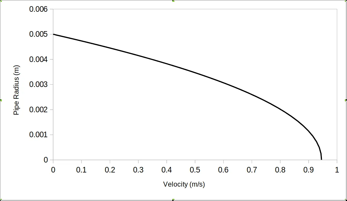
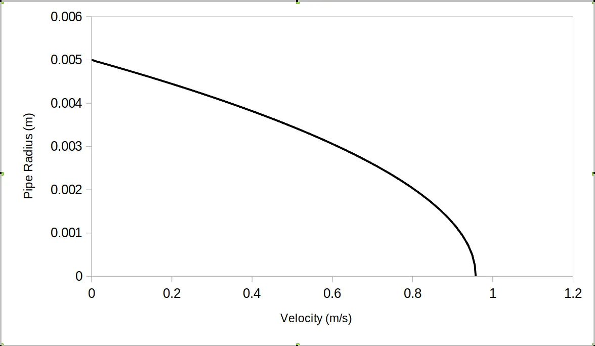
From the plpots below, it is observed that the velocity profile at `x = 0.005` is not parabolic. This shows that the flow is developing in this region. the velocity profiles in the next two locations are both parabolic and almost unchanging, meaning the flow is fully developed.

Wedge angle = 3

The mesh generated for the domains are displayed below for `theta = 3`. The result of the velocity distrbution inside the pipe is also displayed and this is similar to that of `theta = 2`. Velocity profiles observed were similar to those of `theta=2` and they are displayed below.

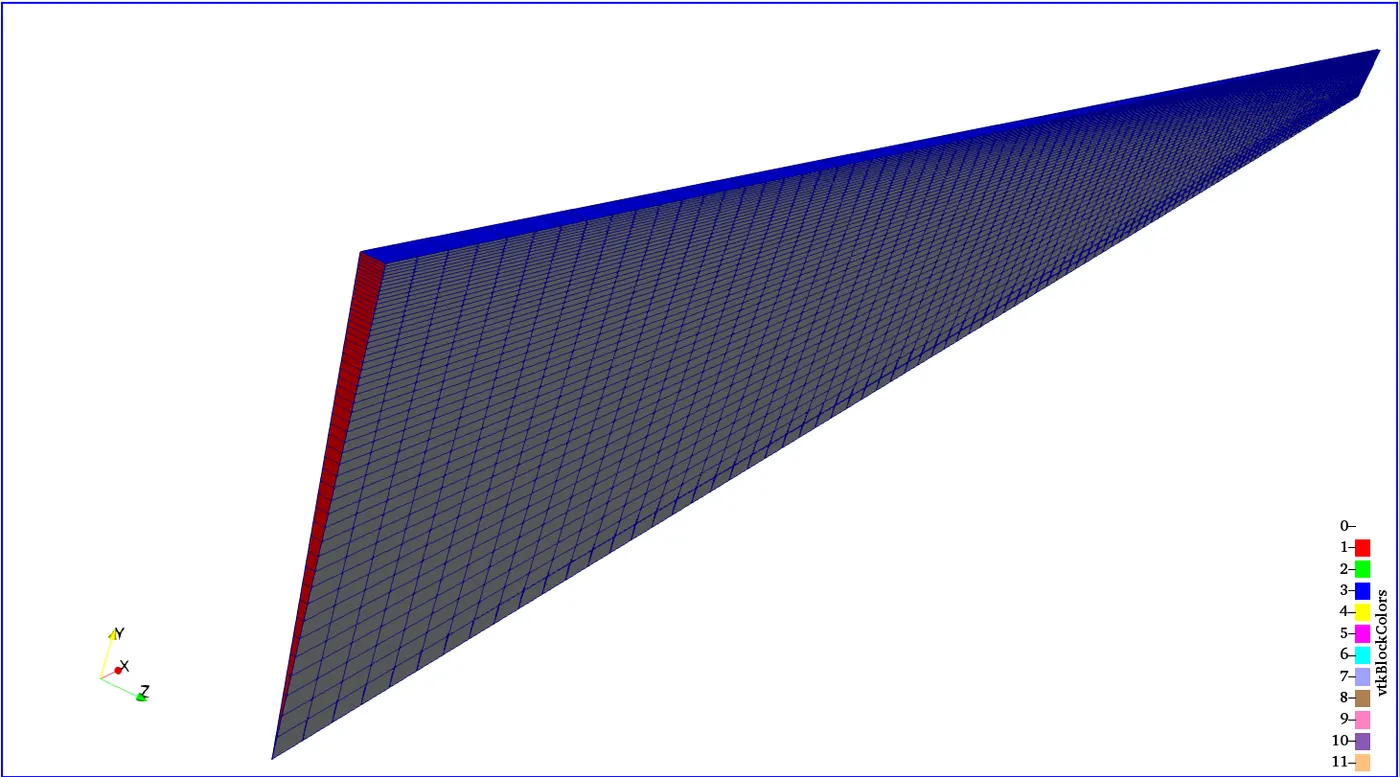
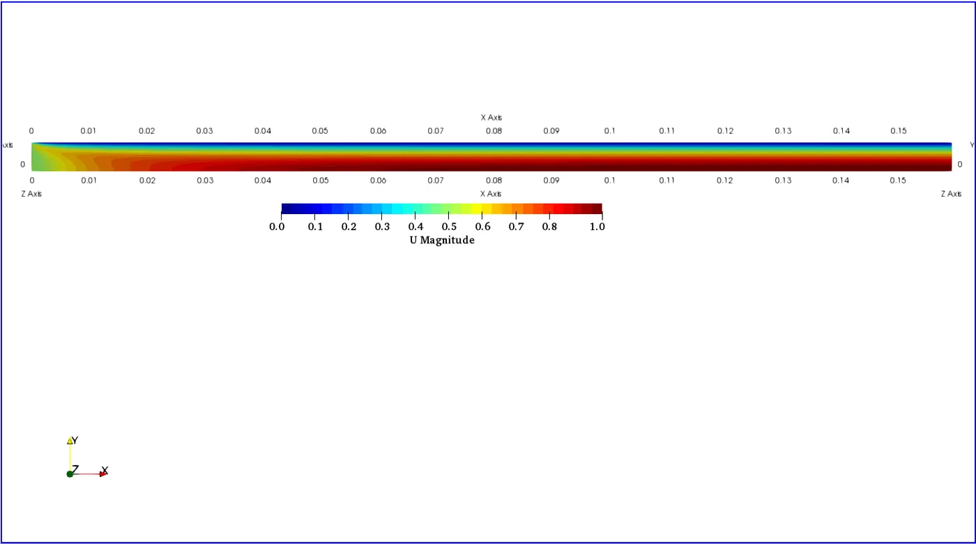
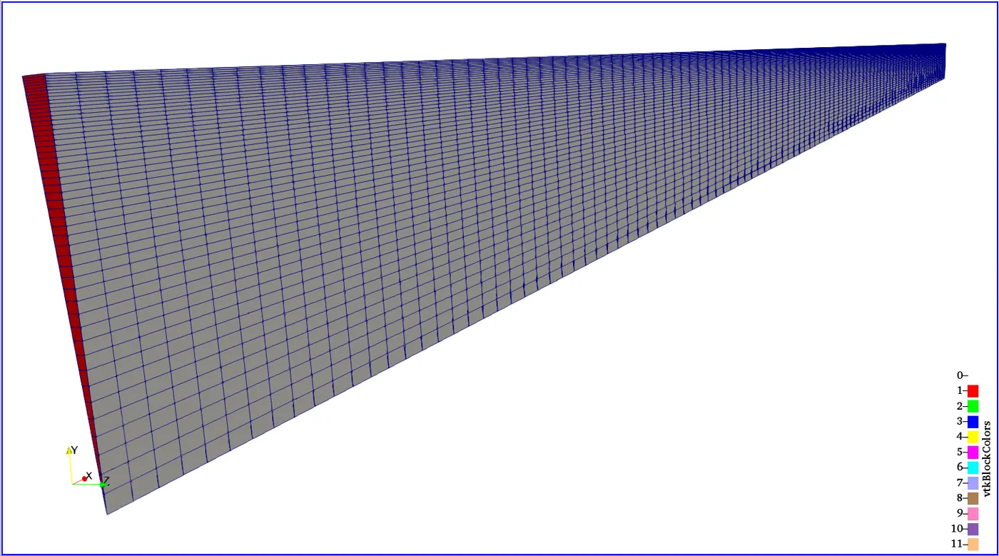
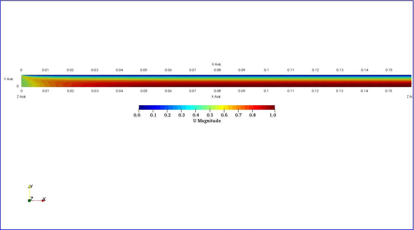
The mesh generated for the domains are displayed below for `theta = 4`. The result of the velocity distrbution inside the pipe is also displayed and this is similar to that of `theta = 2`. Velocity profiles observed were similar to those of `theta=2` and they are displayed below.

Comparing with Analytical Results

The maximum velocities, `u_"max"` at `x=0.155` from the three cases were compared to the maximum velocity from the Hagen-Poiseuille equation. These are tabulated below. The Relative error is calculated as

`"Relative error" = (u_("max", HP) - u_("max", "simulated"))/u_("max", HP) times 100`

Case	`u_("max", simulated)`	`u_("max", HP)`	Relative Error
2	`0.957415`	`0.9600`	`0.269%`
3	`0.957417`	`0.9600`	`0.269%`
4	`0.95742`	`0.9600`	`0.269%`

From the table above, it is observed that the simulated values are `lt 1%` compared to the analytical values.

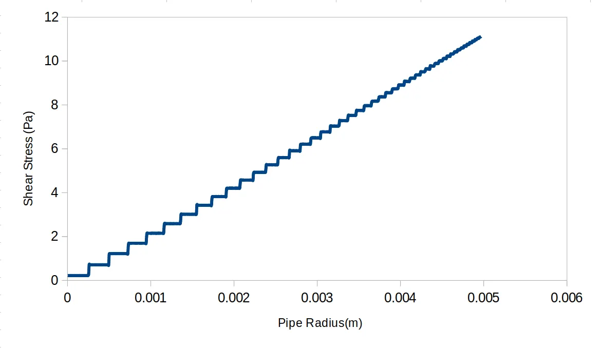
The plot of the shear stress versus pipe radiusat `x=0.0795m` is eqaully displayed below. It is calulate using the formula,

`tau = mu(Deltau)/(Deltar)`

As can be observed, it is near zero at the pipe center and maximum close to the pipe wall. The value at the wall differs from the analytical value by `0.523%`.