Adiabatic Flame Temperature calculation
The AIM and Code is explained in the Coding window.
Introduction
Adiabatic Flame Temperature
Adiabatic flame temperature is the maximum temperature that can be obtained by heating a fuel. Since it is adiabatic, there is no Heat loss.
Adiabatic Flame Temperature can serve as an indicator for comparision of different fuels.
Equivalance Ratio
Equivalance ratio is the ratio between the amount of fuel and air required in a stichiometric condition to amount of fuel and air used.
It is an indicator of how rich or lean a fuel-mixture is.
Code Explanation
Librabries/modules used
import matplotlib.pyplot as plt
import math
import numpy
import cantera
Enthalphy Coeffecients
Enthalphy of a species can be calculated in many ways. Generally, in undergraduate programms enthalphy values are obtained from books called as properties tables of gases or something very similar to that.
In this project, we calculate Enthlphy using the precalculated Enthalphy coeffecients shown below (Source - Berkeley )
# Thermodynamic coeffecients at low temperature (Reactants are at STP = Low Temperature)
# Source - http://combustion.berkeley.edu/gri-mech/version30/files30/thermo30.dat

coeff_N2_l=[0.03298677E+02,0.14082404E-02,-0.03963222E-04,0.05641515E-07,-0.02444854E-10,-0.10208999E+04,0.03950372E+02]
coeff_O2_l=[3.78245636E+00,-2.99673416E-03,9.84730201E-06,-9.68129509E-09,3.24372837E-12,-1.06394356E+03,3.65767573E+00]
coeff_CH4_l=[5.14987613E+00,-1.36709788E-02,4.91800599E-05,-4.84743026E-08,1.66693956E-11,-1.02466476E+04,-4.64130376E+00]
coeff_C2H6_l=[4.29142492E+00,-5.50154270E-03,5.99438288E-05,-7.08466285E-08,2.68685771E-11,-1.15222055E+04,2.66682316E+00]
coeff_C2H4_l=[3.95920148E+00,-7.57052247E-03,5.70990292E-05,-6.91588753E-08,2.69884373E-11,5.08977593E+03,4.09733096E+00]
coeff_C2H2_l=[8.08681094E-01,2.33615629E-02,-3.55171815E-05,2.80152437E-08,-8.50072974E-12,2.64289807E+04,1.39397051E+01]
coeff_C3H8_l=[0.93355381E+00,0.26424579E-01,0.61059727E-05,-0.21977499E-07,0.95149253E-11,-0.13958520E+05,0.19201691E+02]

# Thermodynamic coeffecients at High temperature (Products form at high temperature)

coeff_CO2_h=[3.85746029E+00,4.41437026E-03,-2.21481404E-06,5.23490188E-10,-4.72084164E-14,-4.87591660E+04,2.27163806E+00]
coeff_H2O_h=[3.03399249E+00,2.17691804E-03,-1.64072518E-07,-9.70419870E-11,1.68200992E-14,-3.00042971E+04,4.96677010E+00]
coeff_N2_h=[0.02926640E+02,0.14879768E-02,-0.05684760E-05,0.10097038E-09,-0.06753351E-13,-0.09227977E+04,0.05980528E+02]
coeff_O2_h=[3.28253784E+00,1.48308754E-03,-7.57966669E-07,2.09470555E-10,-2.16717794E-14,-1.08845772E+03,5.45323129E+00]
coeff_CO_h=[2.71518561E+00,2.06252743E-03,-9.98825771E-07,2.30053008E-10,-2.03647716E-14,-1.41518724E+04,7.81868772E+00]
Functions
- Function to calculate the Enthalphy of a species at a specified temperature
def h(T,coeff):			# Enthalpy of Species Calculation

	a1=coeff[0]
	a2=coeff[1]
	a3=coeff[2]
	a4=coeff[3]
	a5=coeff[4]
	a6=coeff[5]
	a7=coeff[6]

	h= (a1 + a2*T/2 + a3*pow(T,2)/3 + a4*pow(T,3)/4 + a5*pow(T,4)/5 + a6/T)*R*T

return h- Function to calculate the difference in Enthalphies at a specified temperature
Here, ER is the equivalance ratio.
def delh(Tg):           # Finding difference in Enthaply of reactants and products at a Temperature


    if ER==1:           #Stichiometric Mixture
        h_reactants = h(T_std,coeff_fuel) + (x+(y/4))*h(T_std,coeff_O2_l) + (x+(y/4))*3.761*h(T_std,coeff_N2_l)
        h_products = x*h(Tg,coeff_CO2_h) + (y/2)*h(Tg,coeff_H2O_h) + (x+(y/4))*3.761*h(Tg,coeff_N2_h)
        delh = h_products - h_reactants

    if ER<1:            #Lean Mixture
        h_reactants = h(T_std,coeff_fuel) + (2/ER)*h(T_std,coeff_O2_l) + (2/ER)*3.761*h(T_std,coeff_N2_l)
        h_products = h(Tg,coeff_CO2_h) + 2*h(Tg,coeff_H2O_h) + ((2/ER)-2)*h(Tg,coeff_O2_h) +(7.52/ER)*h(Tg,coeff_N2_h)
        n_reactants =1+(2/ER)+(2/ER)*3.761
        n_products = 1+2+(2/ER)-2+(7.52/ER)
        delh = h_products - n_products*R*Tguess - h_reactants + n_reactants*R*T_std

    if ER>1:            #Rich Mixture
        h_reactants = h(T_std,coeff_fuel) + (2/ER)*h(T_std,coeff_O2_l) + (2/ER)*3.761*h(T_std,coeff_N2_l)
        h_products = ((4/ER)-3)*h(Tg,coeff_CO2_h) + 2*h(Tg,coeff_H2O_h) + (4-(4/ER))*h(Tg,coeff_CO_h) +(7.52/ER)*h(Tg,coeff_N2_h)
        n_reactants =1+(2/ER)+(2/ER)*3.761
        n_products = (4/ER)-3 + 2 + 4-(4/ER) + (7.52/ER)
        delh = h_products - n_products*R*Tguess - h_reactants + n_reactants*R*T_std

return delh- Function to calculate the difference in Enthalphies when the system is not adiabatic, i.e; there is heat loss term. In this project it is defined as HLF ( Heat Loss Factor)
def delh_HLF(Tg,i):


    if ER==1:                 #Stichiometric Mixture
        h_reactants = h(T_std,coeff_fuel) + (x+(y/4))*h(T_std,coeff_O2_l) + (x+(y/4))*3.761*h(T_std,coeff_N2_l)
        h_products = x*h(Tg,coeff_CO2_h) + (y/2)*h(Tg,coeff_H2O_h) + (x+(y/4))*3.761*h(Tg,coeff_N2_h)
        delh_HLF = (h_products - h_reactants)+802300*i          #LHV of CH4 is 802300

    return delh_HLF
Constants across all the questions
R=8.314 # J/mol k  #Universal Gas Constant
T_std=298.15 #k     #Temperature at STP conditions
tol=1e-4            #Tolerance
alpha = 0.1        #Relaxation Factor
Variation of AFT with ER for CH4 at constant volume using Numerical approach
AFT_ER=[]
ERv=numpy.linspace(0.4,2,30)

for i in ERv:         # For Lean and Rich Mixture

     ER=i
     fuel="C1H4"
     coeff_fuel=coeff_CH4_l
     x=1
     y=4
     j=1
     Tguess=2300

     while abs(delh(Tguess)) >= tol:                 #Newton Raphson Method
            slope = (h(Tguess+tol,coeff_fuel)-h(Tguess,coeff_fuel))/tol
            Tguess=Tguess-alpha*(delh(Tguess)/slope)
            j=j+1

            print(j)

            if j == 20000:
                break

     # print(."Adiabatic Flame Temperature of %s at ER %d is %dk"% (fuel,ER,Tguess))

     AFT_ER.append(Tguess)

plt.plot(ERv,AFT_ER,'-o',color='r',label='Python_Numerical')
plt.grid()
plt.xlabel("Equivalence Ratio")
plt.ylabel("Adiabatic Fuel Temperature")
Variation of AFT with ER for CH4 at constant volume using Cantera Module/Library
gas=cantera.Solution('gri30.xml')
AFT_CT=[]

for i in ERv:

    nTotal=1+(2/i)+(7.52/i)

    gas.TPX=298.15,101325,{'CH4':1/nTotal,'O2':(2/i)/nTotal,'N2':(7.52/i)/nTotal}

    gas.equilibrate('UV')

    AFT_CT.append(gas.T)

plt.plot(ERv,AFT_CT,'-*',color='b',label='Cantera')
plt.legend()
plt.show()
Result
Comparision of AFT vs ER obtained from Python and Cantera
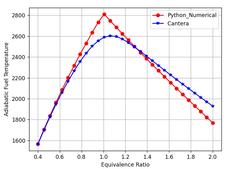
(** Adiabatic Final Temperature - Mentioned incorrectly on y-label in the above plot)
Inference
- It can be seen that the AFT values are different when obtained from Numerical approach and from Cantera. This is because Cantera takes into consideration all the additional products that are formed during the reaction, for example CN, NC, HCO, although these are formed in very less quanitities, they consume considerable amount of energy in their formation and thus decreasing the Adiabatic Final Temperature. Thus, generally Cantera Minimises the AFT values and they are more close to the values obtained experimentally.
- The values of AFT for Rich Mixture are higher in Cantera. I am not sure why is that. But I geuss It has to do something with the intermediate reactions.
Variation of AFT wrt HLF for CH4 at constant pressure
ER=1
coeff_fuel=coeff_CH4_l
x=1
y=4
Tguess=2000
Tg=2000

HLF=numpy.linspace(0,1,10)

AFT_HLF=[]

for i in HLF:
     j=1
     while abs(delh_HLF(Tguess,i)) > tol:                 #Newton Raphson Method
            slope = (h(Tguess+tol,coeff_fuel)-h(Tguess,coeff_fuel))/tol
            Tguess=Tguess-alpha*(delh_HLF(Tguess,i)/slope)
            j=j+1

     AFT_HLF.append(Tguess)
plt.plot(HLF,AFT_HLF,'-*')
plt.grid()
plt.xlabel("Heat Loss Factor")
plt.ylabel("Adiabatic Fuel Temperature")
plt.show()
Result
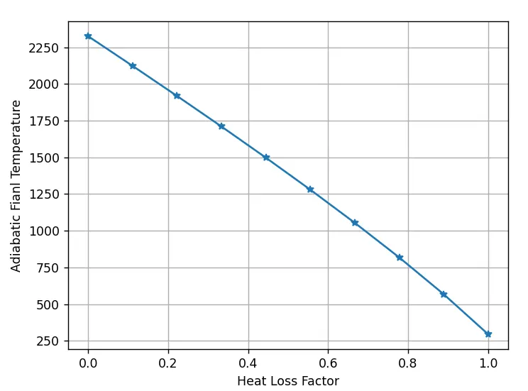
Variation of AFT wrt HLF
Inference
- The plot shown above is pretty self-explanatory.
- As the Heat Loss increases, the Adiabatic Flame Temeprature decreases.
Variation of AFT for different species
options=["C2H2","C1H4","C2H6","C3H8","C2H4"]
# options=["C2H2"]
AFT=[]

for i in range(0,len(options)):          # Using for loop to calculate AFT for all species, so as to create a plot.

        fuel=options[i]
        x=int(options[i][1])
        y=int(options[i][3])
        ER=1

        if fuel=="C1H4":
            coeff_fuel=coeff_CH4_l

        if fuel=="C2H6":
            coeff_fuel=coeff_C2H6_l

        if fuel=="C3H8":
            coeff_fuel=coeff_C3H8_l

        if fuel=="C2H4":
            coeff_fuel=coeff_C2H4_l

        if fuel=="C2H2":
            coeff_fuel=coeff_C2H2_l

        Tguess = 2300		#initial guess value for Adiabatic Flame Temperature
        j=1

        while abs(delh(Tguess)) >= tol:                 #Newton Raphson Method
            slope = (h(Tguess+tol,coeff_fuel)-h(Tguess,coeff_fuel))/tol
            Tguess=Tguess-alpha*(delh(Tguess)/slope)
            j=j+1
            #plt.plot(j,Tguess,'*',color='r')

        #plt.show()

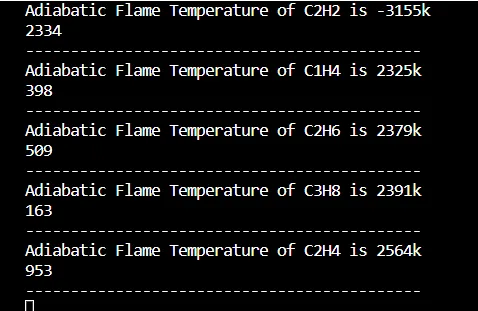
        print("Adiabatic Flame Temperature of %s is %dk"% (fuel,Tguess))
        print(j)
        #print(slope)
        print('--------------------------------------------')
        AFT.append(Tguess)


Q3=[options[1]]+options[3:]
QA3=[AFT[1]]+AFT[3:]

Q4=options[0:3]
QA4=AFT[0:3]

plt.plot(Q4,QA4,color='r',label='Carbon atoms')
plt.plot(Q3,QA3,color='b',label='Carbon bonds')
plt.grid()
plt.legend()

plt.xlabel("Hydrocarbon")
plt.ylabel("Adiabatic Fuel Temperature")
plt.show()
Result
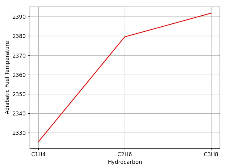
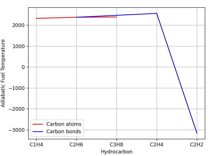
Inference:
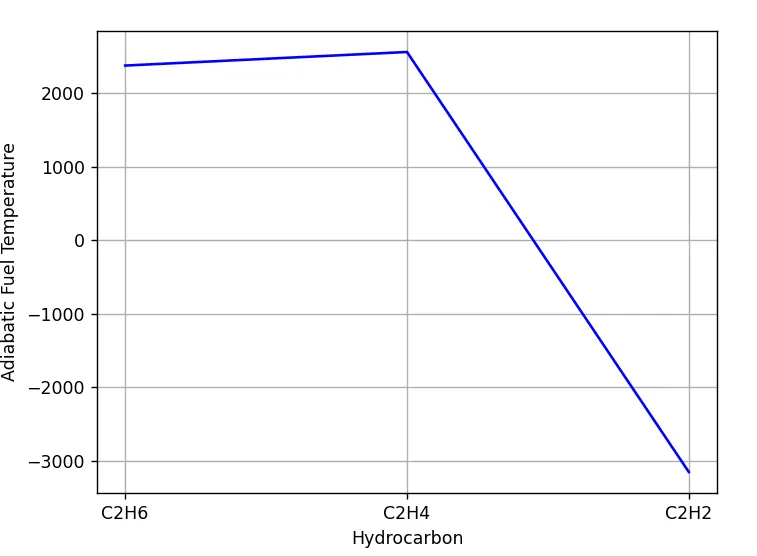
- As the number of carbon atoms in a hydrocarbon increases, the AFT increases. This is understandable as more the number of carbon atoms more the amount of energy stored in the fuel. Although it also depends on the structure of the compound.
- The value obtained for C2H2 is incorrect and am still trying to figure out why is that. Changing the relaxation factor also isnt helping much here. Once the error is clear, it will be updated here. Meanwhile if the reader is able to spot the error, please mention it in the comments section.
Cumulative Code:
Caution - Unindent the required parts before running the code
'''
 -------------------------------------------- KRISHNA MUNDADA -----------------------------------------------------------
1) Plot AFT Vs Equivalance Ratio for CH4 at Constant Volume using Numerical approach and Cantera appraoch
2) Plot AFT Vs Heat loss Factor for CH4 at Constant Pressure
3 and 4 ) plot ADT for the given Species
-------------------------------------------------------------------------------------------------------------------------
'''

import matplotlib.pyplot as plt
import math
import numpy
import cantera

# Thermodynamic coeffecients at low temperature (Reactants are at STP = Low Temperature)
# Source - http://combustion.berkeley.edu/gri-mech/version30/files30/thermo30.dat

coeff_N2_l=[0.03298677E+02,0.14082404E-02,-0.03963222E-04,0.05641515E-07,-0.02444854E-10,-0.10208999E+04,0.03950372E+02]
coeff_O2_l=[3.78245636E+00,-2.99673416E-03,9.84730201E-06,-9.68129509E-09,3.24372837E-12,-1.06394356E+03,3.65767573E+00]
coeff_CH4_l=[5.14987613E+00,-1.36709788E-02,4.91800599E-05,-4.84743026E-08,1.66693956E-11,-1.02466476E+04,-4.64130376E+00]
coeff_C2H6_l=[4.29142492E+00,-5.50154270E-03,5.99438288E-05,-7.08466285E-08,2.68685771E-11,-1.15222055E+04,2.66682316E+00]
coeff_C2H4_l=[3.95920148E+00,-7.57052247E-03,5.70990292E-05,-6.91588753E-08,2.69884373E-11,5.08977593E+03,4.09733096E+00]
coeff_C2H2_l=[8.08681094E-01,2.33615629E-02,-3.55171815E-05,2.80152437E-08,-8.50072974E-12,2.64289807E+04,1.39397051E+01]
coeff_C3H8_l=[0.93355381E+00,0.26424579E-01,0.61059727E-05,-0.21977499E-07,0.95149253E-11,-0.13958520E+05,0.19201691E+02]

# Thermodynamic coeffecients at High temperature (Products form at high temperature)

coeff_CO2_h=[3.85746029E+00,4.41437026E-03,-2.21481404E-06,5.23490188E-10,-4.72084164E-14,-4.87591660E+04,2.27163806E+00]
coeff_H2O_h=[3.03399249E+00,2.17691804E-03,-1.64072518E-07,-9.70419870E-11,1.68200992E-14,-3.00042971E+04,4.96677010E+00]
coeff_N2_h=[0.02926640E+02,0.14879768E-02,-0.05684760E-05,0.10097038E-09,-0.06753351E-13,-0.09227977E+04,0.05980528E+02]
coeff_O2_h=[3.28253784E+00,1.48308754E-03,-7.57966669E-07,2.09470555E-10,-2.16717794E-14,-1.08845772E+03,5.45323129E+00]
coeff_CO_h=[2.71518561E+00,2.06252743E-03,-9.98825771E-07,2.30053008E-10,-2.03647716E-14,-1.41518724E+04,7.81868772E+00]

# 'CxHy + (x + y/4)*(0.21 O2 + 0.79 N2)  --> x Co2 + y/2 H2o + (x + y/4)*(0.79) N2 --> Balanced Stichiometric Equation


def h(T,coeff):			# Enthalpy of Species Calculation

	a1=coeff[0]
	a2=coeff[1]
	a3=coeff[2]
	a4=coeff[3]
	a5=coeff[4]
	a6=coeff[5]
	a7=coeff[6]

	h= (a1 + a2*T/2 + a3*pow(T,2)/3 + a4*pow(T,3)/4 + a5*pow(T,4)/5 + a6/T)*R*T

	return h

def delh(Tg):           # Finding difference in Enthaply of reactants and products at a Temperature


    if ER==1:           #Stichiometric Mixture
        h_reactants = h(T_std,coeff_fuel) + (x+(y/4))*h(T_std,coeff_O2_l) + (x+(y/4))*3.761*h(T_std,coeff_N2_l)
        h_products = x*h(Tg,coeff_CO2_h) + (y/2)*h(Tg,coeff_H2O_h) + (x+(y/4))*3.761*h(Tg,coeff_N2_h)
        delh = h_products - h_reactants

    if ER<1:            #Lean Mixture
        h_reactants = h(T_std,coeff_fuel) + (2/ER)*h(T_std,coeff_O2_l) + (2/ER)*3.761*h(T_std,coeff_N2_l)
        h_products = h(Tg,coeff_CO2_h) + 2*h(Tg,coeff_H2O_h) + ((2/ER)-2)*h(Tg,coeff_O2_h) +(7.52/ER)*h(Tg,coeff_N2_h)
        n_reactants =1+(2/ER)+(2/ER)*3.761
        n_products = 1+2+(2/ER)-2+(7.52/ER)
        delh = h_products - n_products*R*Tguess - h_reactants + n_reactants*R*T_std

    if ER>1:            #Rich Mixture
        h_reactants = h(T_std,coeff_fuel) + (2/ER)*h(T_std,coeff_O2_l) + (2/ER)*3.761*h(T_std,coeff_N2_l)
        h_products = ((4/ER)-3)*h(Tg,coeff_CO2_h) + 2*h(Tg,coeff_H2O_h) + (4-(4/ER))*h(Tg,coeff_CO_h) +(7.52/ER)*h(Tg,coeff_N2_h)
        n_reactants =1+(2/ER)+(2/ER)*3.761
        n_products = (4/ER)-3 + 2 + 4-(4/ER) + (7.52/ER)
        delh = h_products - n_products*R*Tguess - h_reactants + n_reactants*R*T_std

    return delh

def delh_HLF(Tg,i):


    if ER==1:                 #Stichiometric Mixture
        h_reactants = h(T_std,coeff_fuel) + (x+(y/4))*h(T_std,coeff_O2_l) + (x+(y/4))*3.761*h(T_std,coeff_N2_l)
        h_products = x*h(Tg,coeff_CO2_h) + (y/2)*h(Tg,coeff_H2O_h) + (x+(y/4))*3.761*h(Tg,coeff_N2_h)
        delh_HLF = (h_products - h_reactants)+802300*i          #LHV of CH4 is 802300

    return delh_HLF


R=8.314 # J/mol k  #Universal Gas Constant
T_std=298.15 #k     #Temperature at STP conditions
tol=1e-4            #Tolerance
alpha = 0.1        #Relaxation Factor

'''
# *************************** Question 1 *****************************

AFT_ER=[]
ERv=numpy.linspace(0.4,2,30)

for i in ERv:         # For Lean and Rich Mixture

     ER=i
     fuel="C1H4"
     coeff_fuel=coeff_CH4_l
     x=1
     y=4
     j=1
     Tguess=2300

     while abs(delh(Tguess)) >= tol:                 #Newton Raphson Method
            slope = (h(Tguess+tol,coeff_fuel)-h(Tguess,coeff_fuel))/tol
            Tguess=Tguess-alpha*(delh(Tguess)/slope)
            j=j+1

            print(j)

            if j == 20000:
                break

     # print(."Adiabatic Flame Temperature of %s at ER %d is %dk"% (fuel,ER,Tguess))

     AFT_ER.append(Tguess)

plt.plot(ERv,AFT_ER,'-o',color='r',label='Python_Numerical')
plt.grid()
plt.xlabel("Equivalence Ratio")
plt.ylabel("Adiabatic Fuel Temperature")

gas=cantera.Solution('gri30.xml')
AFT_CT=[]

for i in ERv:

    nTotal=1+(2/i)+(7.52/i)

    gas.TPX=298.15,101325,{'CH4':1/nTotal,'O2':(2/i)/nTotal,'N2':(7.52/i)/nTotal}

    gas.equilibrate('UV')

    AFT_CT.append(gas.T)

plt.plot(ERv,AFT_CT,'-*',color='b',label='Cantera')
plt.legend()
plt.show()

'''
# *************************    Question 2    ********************************
'''
ER=1
coeff_fuel=coeff_CH4_l
x=1
y=4
Tguess=2000
Tg=2000

HLF=numpy.linspace(0,1,10)

AFT_HLF=[]

for i in HLF:
     j=1
     while abs(delh_HLF(Tguess,i)) > tol:                 #Newton Raphson Method
            slope = (h(Tguess+tol,coeff_fuel)-h(Tguess,coeff_fuel))/tol
            Tguess=Tguess-alpha*(delh_HLF(Tguess,i)/slope)
            j=j+1

     AFT_HLF.append(Tguess)
plt.plot(HLF,AFT_HLF,'-*')
plt.grid()
plt.xlabel("Heat Loss Factor")
plt.ylabel("Adiabatic Fianl Temperature")
plt.show()

'''
# **************************  Question 3 and 4 ****************************
'''
options=["C1H4","C2H6","C3H8","C2H4","C2H2"]
# options=["C2H2"]
AFT=[]

for i in range(0,len(options)):          # Using for loop to calculate AFT for all species, so as to create a plot.

        fuel=options[i]
        x=int(options[i][1])
        y=int(options[i][3])
        ER=1

        if fuel=="C1H4":
            coeff_fuel=coeff_CH4_l

        if fuel=="C2H6":
            coeff_fuel=coeff_C2H6_l

        if fuel=="C3H8":
            coeff_fuel=coeff_C3H8_l

        if fuel=="C2H4":
            coeff_fuel=coeff_C2H4_l

        if fuel=="C2H2":
            coeff_fuel=coeff_C2H2_l

        Tguess = 2300		#initial guess value for Adiabatic Flame Temperature
        j=1

        while abs(delh(Tguess)) >= tol:                 #Newton Raphson Method
            slope = (h(Tguess+tol,coeff_fuel)-h(Tguess,coeff_fuel))/tol
            Tguess=Tguess-alpha*(delh(Tguess)/slope)
            j=j+1
            #plt.plot(j,Tguess,'*',color='r')

        #plt.show()

        print("Adiabatic Flame Temperature of %s is %dk"% (fuel,Tguess))
        print(j)
        #print(slope)
        print('--------------------------------------------')
        AFT.append(Tguess)


Q3=[options[1]]+options[3:]
QA3=[AFT[1]]+AFT[3:]

Q4=options[0:3]
QA4=AFT[0:3]

plt.plot(Q4,QA4,color='r',label='Carbon atoms')
plt.grid()
plt.xlabel("Hydrocarbon")
plt.ylabel("Adiabatic Fuel Temperature")
plt.show()

plt.plot(Q3,QA3,color='b',label='Carbon bonds')
plt.grid()
plt.xlabel("Hydrocarbon")
plt.ylabel("Adiabatic Fuel Temperature")
plt.show()


plt.plot(Q4,QA4,color='r',label='Carbon atoms')
plt.plot(Q3,QA3,color='b',label='Carbon bonds')
plt.grid()
plt.xlabel("Hydrocarbon")
plt.ylabel("Adiabatic Fuel Temperature")
plt.legend()
plt.show()

'''