Week 3 - Adiabatic Flame Temperature calculation

Week 3 - Adiabatic Flame Temperature calculation :

Objectives :

1. Adiabatic flame temperature variation with Equivalence ratio (In constant volume-chamber)

2. Flame temperature variation with Heat loss (In constant pressure-chamber)

3. Adiabatic flame temperature variation with respect to Alkane, Alkene, Alkyne

4. Adiabatic flame temperature variation with respect to number of Carbon atom chains

Theory :

It is a chemical process in which a substance (fuel) reacts rapidly with an oxidiser to release energy. The fuel can be a solid, liquid or gas.

Adiabatic Flame Temprature :

When a combustion reaction takes place energy is released to the combustion products, if no heats is lost in the process or the combustion chamber is adiabatic the temprature of the combustion products is known as "Adiabatic Flame Temprature".

In a combustion process energy in the form of heat is produced and this heat increases the temprature of the combustion products inside the combustion chamber. Since, it is an adiabatic combustion chamber there is no heat loss to the surrounding. As a result, the temprature of products inside the chamber increased. The highest temprature is known as Adiabatic Flame Temprature.

The temprature rise inside a combustion chamber depends on the air-fuel ratio.For example, when we use excess oxideiser, the flame temprature is determined from the energy balance of the reaction at equilbrium. There are two types of adiabatic flame temprature.

• Constant Pressure Adiabatic Flame Temprature
• Constant Volume Adiabatic Flame Temprature

Adiabatic Flame Temprature Calculation :

Theoretically, AFT can be obtained by equilaizing the enthalpies of products and reactants. We are going to use a polynomial function from the database of NASA at a particular temprature.

h(T) =`(a1 + a2.(T/2) + a3.((T^2)/3) + a4.((T^3)/4) + a5.((T^4)/5) + a6.(T/6))*R*T`

where,

h =enthalpy

ai =coefficient of each species

T =Temprature

R =Gas Constant

The co-efficient, values can be extracted from the websites of the GRI MECH 30, thermostat file. For the reactants, we take low temprature i.e; STP conditions and for the products usually, temprature are high.

The AFT is calculated using Newton's Raphson iterative technique where an initial guess value for the temprature is assumednand it iterates until it reaches the prescribed tolerance value.

`T_(New) = T_(guess) -alpha[f(T_(guess))/(f'(T_(guess)))]`

where,

`T_(New)`= New value of the temprature after the successive iterative

`T_(guess)` =Initial guess temprature

`alpha` = Relaxation Factor(< 1 under relaxed,>1 over relaxed)

Combustion Stoichiometry :

Stoichiometric Mixture contains the exact amount of fuel and oxidizer such that complete combustion takes place where all the fuels and oxidizer are consumed to form the products. The mixture ideally yields the maximum flame temprature as all the energy released from the combustion is used to heat the products.

The Stoichiometric Combustion equations for methane air is:

`CH_4 + 2(O_2 + 3.76 N_2) -> CO_2 + 2H_2O + 7.52N_2`

In general for the class of Hydrocarbons, we can express the stoichiometric equation as follows :-

`C_xH_y + (x + y/4)CO_2 + 3.76N_2) -> xCO_2 + (y/2)H_2O + (x + y/4)N_2`

When the fuel is not getting burned completely, we obtain products such as `O_2`, `H_2`, CO, OH, etc. In practice it is hard to find a combustion process equal to stoichiometry conditions. If less air is used the mixture is defined as the fuel-rich mixture and a common notation to represent this ratio is the equivalence ratio (`phi`).

The equivalence ratio is the ratio of the actual fuel-air ratio to the stoichiometric ratio. Hence, if `phi`<1 the mixture is lean and if `phi`>1 the mixture is rich.

For Lean Mixture :-

`CH_4 + (2/phi)(O_2 + 3.76N_2) -> CO_2 + 2H_2O + (2/phi-2) O_2 + 7.5/phi.N_2`

For Rich Mixture :-

`CH_4 + 2/phi(O_2 + 3.76N_2) -> (4/phi-3)CO_2 + 2H_2O + (4-4/phi)CO_2 + 7.52/phi.N_2`

CASE 1 :

The Adiabatic Flame Temprature (AFT) of methane-air combustion with different equivalence ratio's using the constant volume chamber. This result is validated using the data from CANTERA.

Program for Ist case :-

'''
Program to study the dependance of Adiabatic Flame Temprature on Equivalence Ratio

Rich Mixture(phi>1): CH4 + (2/phi)(O2 + 3.76N2) <=> (4/phi - 3)CO2 + 2H2O + (7.52/phi)N2 + (4 - 4/phi)CO
Lean Mixture(phi<1): CH4 + (2/phi)(O2 + 3.76N2) <=> CO2 + 2H2O + (7.52/phi)N2 + (2/phi - 2)O2

Here, phi is the equivalence ratio i.e; given fuel-air ratio to stotichiometric fuel-air ratio

The above calculations are assumed from the solved equation below 

A stoichometric mixture of combustion of methane looks like the following 

CH4 +2(O2 + 3.76N2) --> CO2 + 2H2O + 7.52N2

A lean mixture of combustion of methane has an extra oxygen atom formal in the product side:

CH4 + x(O2 + 3.76N2) --> aCO2 + bH2O + 3.76xN2 + cO2

Comparing co-efficient on b.s. a=1; 2b=4 -> b=2; Also if equivalence ratio = Φ and fuel mole =1, then x =2/Φ. Hence the equation becomes 

CH4 + 2/Φ(O2 + 3.76N2) --> CO2 + 2H2O + 7.52 /ΦN2 + cO2

On comparing both sides we get c = 2/Φ - 2

CH4 + 2/Φ(O2 + 3.76N2) --> aCO2 + 2H2O + 7.52/ΦN2 + dCO

Now comparing we get a =4/Φ -3 and d= 4-4/Φ.

CH4 + 2/Φ(O2 + 3.76N2) --> (4/Φ - 3)CO2 + 2H2O + 7.52 /ΦN2 + (4-4/Φ)CO  


'''

import matplotlib.pyplot as plt
import cantera as ct
# Function defining temprature and co-efficient
def h(T, coeff):
	R =8.314 #J/mol-K

	a1 =coeff[0]
	a2 =coeff[1]
	a3 =coeff[2]
	a4 =coeff[3]
	a5 =coeff[4]
	a6 =coeff[5]

	return (a1 + a2*(T/2) + a3*pow(T,2)/3 + a4*pow(T,3)/4 + a5*pow(T,4)/5 + a6/T )*R*T

# Defining the NASA co-efficient from datasheet of reactant (low temprature)

ch4_coeff_l =[5.14987613E+00, -1.36709788E-02, 4.91800599E-05, -4.84743026E-08, 1.66693956E-11, -1.02466476E+04, -4.64130376E+00]
o2_coeff_l =[3.78245636E+00, -2.99673416E-03, 9.84730201E-06, -9.68129509E-09, 3.24372837E-12, -1.06394356E+03,  3.65767573E+00 ]
n2_coeff_l =[0.03298677E+02, 0.14082404E-02, -0.03963222E-04,  0.05641515E-07, -0.02444854E-10, -0.10208999E+04, 0.03950372E+02 ]

# Defining the NASA co-efficient from datasheet of reactant (high temprature)

co2_coeff_h =[3.85746029E+00, 4.41437026E-03, -2.21481404E-06, 5.23490188E-10, -4.72084164E-14, -4.87591660E+04, 2.27163806E+00]
h2o_coeff_h =[3.03399249E+00, 2.17691804E-03, -1.64072518E-07, -9.70419870E-11, 1.68200992E-14, -3.00042971E+04, 4.96677010E+00]
n2_coeff_h =[0.02926640E+02, 0.14879768E-02, -0.05684760E-05, 0.10097038E-09, -0.06753351E-13, -0.09227977E+04, 0.05980528E+02]
co_coeff_h =[2.71518561E+00, 2.06252743E-03, -9.98825771E-07, 2.30053008E-10, -2.03647716E-14, -1.41518724E+04, 7.81868772E+00]
o2_coeff_h =[3.28253784E+00, 1.48308754E-03, -7.57966669E-07, 2.09470555E-10, -2.16717794E-14, -1.08845772E+03, 5.45323129E+00]

# Defining the function for root solving by Newton Raphson method
def f(T,phi):
	Tstp =298.15 #Temprature of the reactant in Kelvin
	R =8.314 #J/mol-K
	h_ch4_r =h(Tstp, ch4_coeff_l)
	h_o2_r =h(Tstp, o2_coeff_l)
	h_n2_r =h(Tstp, n2_coeff_l)

	H_reactants =h_ch4_r + (2/phi)*h_o2_r + (7.52/phi)*h_n2_r
	N_reactants =(1 + (2/phi) + (7.52/phi))*R*Tstp

	h_co2_p =h(T, co2_coeff_h)
	h_h2o_p =h(T, h2o_coeff_h)
	h_n2_p =h(T, n2_coeff_h)
	h_co_p =h(T, co_coeff_h)
	h_o2_p =h(T, o2_coeff_h)

	if phi >= 1:
		H_products =(4/phi-3)*h_co2_p + 2*h_h2o_p + (7.52/phi)*h_n2_p + (4-4/phi)*h_co_p
		N_products =((4/phi-3) + 2 + (7.52/phi) + (4-4/phi))*R*T

	elif phi < 1:
		H_products =h_co2_p + 2*h_h2o_p + (7.52/phi)*h_n2_p + (2/phi-2)*h_o2_p
		N_products =(1 + 2 + (7.52/phi) + (2/phi-2))*R*T

	return (H_products - H_reactants) - (N_products - N_reactants)
	
# Since reaction is in a constant volume chamber no. of moles are also added

def fprime(T, phi):
	return (f(T+1e-6, phi) - f(T,phi))/(1e-6)


# Defining Newton-Raphson solver 

alpha =0.2
tol =1e-3
phi =[0.1, 0.2, 0.3, 0.4, 0.5, 0.6, 0.7, 0.8, 0.9, 1, 1.1, 1.2, 1.3, 1.4, 1.5, 1.6, 1.7, 1.8, 1.9, 2]
T_aft_py =[]


for i in range(0, len(phi)):
	T_guess =1500 # K
	while abs(f(T_guess, phi[i])) >= tol:
		T_guess =T_guess -alpha*((f(T_guess, phi[i]))/(fprime(T_guess, phi[i])))
	T_aft_py.append(T_guess)
print(T_aft_py)
print()

'''
Solution obtained by Cantera
'''

gas =ct.Solution('gri30.xml')
T_aft_ct =[]

for i in range(0, len(phi)):
	# Computing the mole fractions of each reactant
	n_tot =1 + (2/phi[i]) + (7.52/phi[i])
	n_ch4 =1/n_tot
	n_o2 =(2/phi[i])/n_tot
	n_n2 =(7.52/phi[i])/n_tot
	# Defining the gas mixture
	gas.TPX =298.15, 101325,{'CH4':n_ch4, 'O2':n_o2, 'N2':n_n2}
	# Calculating the equilbrium conditions
	gas.equilibrate('UV','auto')
	T_aft_ct.append(gas.T)
print(T_aft_ct)


# Plotting the results
plt.plot(phi,T_aft_py,'-o',color='red',label='Python')
plt.plot(phi,T_aft_ct,'-o',color='blue',label='Cantera')
plt.xlabel('Equivalence Ratio ($phi$)', fontsize=14)
plt.ylabel('Adiabatic Flame Temprature [K]',fontsize=14)
plt.grid('on')
plt.title('AFT vs. Equivalence Ratio for Methane Air Combustion',fontsize=16,fontweight='bold')
plt.legend(fontsize=14)
plt.show() 	

Results :

CASE II :

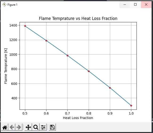
Effect of loss of heat on Adiabatic Flame Temprature is in a Constant Pressure Chamber :

In case, we are considering the heat loss phenomenon in a constant pressure chamber. The reaction is not adiabatic hence there will be a loss of heat from the system to the outside world. The reaction will be considering is the stoichiometric combustion of Methane-Air :

`CH_4 + 2(O_2 + 3.76N_2) -> CO_2 + 2H_2O + 7.52N_2`

The maximum possible heat loss is going to be calculated using the Lower Heating Value (LHV). The heat loss factor is varied from no heat loss to 0.5 i.e; 50% heat loss as a multiplier of LHV. Heat Loss is an additive to the difference between the enthalpy of products and reactants.

Program for IInd Case :-

import matplotlib.pyplot as plt

 # Stoichiometric reaction : CH4 + 2(O2 + 3.76N2) -> CO2 + 2H20 + 7.52N2

 # Function defining temprature and co- efficients
def h(T, coeffs):

 	R =8.314 #J/mol-K
 	a1 =coeffs[0]
 	a2 =coeffs[1]
 	a3 =coeffs[2]
 	a4 =coeffs[3]
 	a5 =coeffs[4]
 	a6 =coeffs[5]

 	return (a1 + a2*(T/2) + a3*pow(T,2)/3 + a4*pow(T,3)/4 + a5*pow(T,4)/5 + a6/T )*R*T

# Defining the NASA co-efficients from datasheet of reactants (low temprature)

ch4_coef_l =[5.14987613E+00, -1.36709788E-02, 4.91800599E-05, -4.84743026E-08, 1.66693956E-11, -1.02466476E+04, -4.64130376E+00]
o2_coef_l =[3.78245636E+00, -2.99673416E-03, 9.84730201E-06, -9.68129509E-09, 3.24372837E-12, -1.06394356E+03, 3.65767573E+00]
n2_coef_l =[0.03298677E+02, 0.14082404E-02, -0.03963222E-04, 0.05641515E-07, -0.02444854E-10, -0.10208999E+04, 0.03950372E+02]

# Defining the NASA coefficient from datasheet of reactants (high temprature)

n2_coef_h  =[0.02926640E+02, 0.14879768E-02, -0.05684760E-05, 0.10097038E-09, -0.06753351E-13, -0.09227977E+04, 0.05980528E+02]
h2o_coef_h =[3.03399249E+00, 2.17691804E-03, -1.64072518E-07, -9.70419870E-11, 1.68200992E-14, -3.00042971E+04, 4.96677010E+00]
co2_coef_h =[3.85746029E+00, 4.41437026E-03, -2.21481404E-06, 5.23490188E-10, -4.72084164E-14, -4.87591660E+04, 2.27163806E+00]

# Computing the maximum possible heat loss
Tstd =298.15
LHV =h(Tstd, ch4_coef_l) + 2*h(Tstd, o2_coef_l) - h(Tstd, co2_coef_h) - 2*h(Tstd, h2o_coef_h) # Nitrogen gets cancelled as the same moles in reactant and product side

# Evaluation of enthalpy
def f(T, H_loss):
	Tstd =298.15 

	#Enthalpy of products
	h_co2_p =h(T, co2_coef_h)
	h_h2o_p =h(T, h2o_coef_h)
	h_n2_p =h(T, n2_coef_h)
	H_p =h_co2_p + 2*h_h2o_p + 7.52*h_n2_p

	#print(H_p)
	#enthalpy of reactants
	h_ch4_r =h(Tstd, ch4_coef_l)
	h_o2_r = h(Tstd, o2_coef_l)
	h_n2_r = h(Tstd, n2_coef_l)
	H_r    =h_ch4_r + 2*h_o2_r + 7.52*h_n2_r

	#print(H_r)
	print(LHV)
	return H_p - H_r + (H_loss *LHV)

def fprime(T):
	return (f(T + 1e-6, H_loss) -f(T, H_loss))/1e-6

H_loss =0.5
T_aft =[]
H_l =[]

while(H_loss < 1):
	T_g =1500
	tol =1e-4
	alpha =1
	ct =0
# Newton Raphson technique
	while (abs(f(T_g, H_loss)) >tol):
		T_g =T_g - alpha*((f(T_g, H_loss)/fprime(T_g)))
		ct =ct + 1
	plt.plot(H_loss, T_g,'*',color='red')
	H_l.append(H_loss)
	H_loss =H_loss +0.1
	T_aft.append(T_g)

plt.plot(H_l, T_aft)
plt.xlabel('Heat Loss Fraction')
plt.ylabel('Flame Temprature [K]')
plt.title('Flame Temprature vs Heat Loss Fraction')
plt.grid(True)
plt.show()		 	

Result :

CASE III :

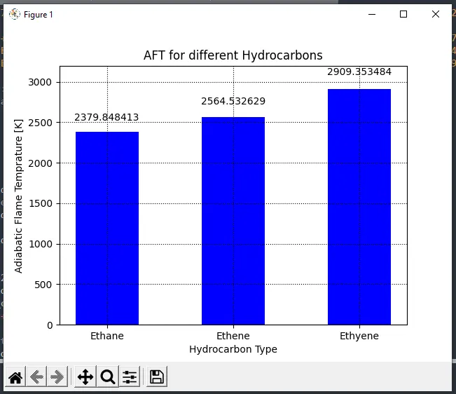
Effects of fuel type (Alkanes, Alkenes and Alkyene) on adiabatic flame temprature with 0% Heat Loss.

In this CASE, we will be examining the AFT of Alkane (Ethane(, Alkene(Ethene), and Alkyene(Ethyene). We will be writing a code considering a heat loss of 0%.

ETHANE :

`C_2H_6 + 3.5(O_2 + 3.76N_2) -> 2CO_2 + 3H_2O + 3.5(3.76N_2)`

ETHENE:

`C_2H_4 + 3(O_2 + 3.76N_2) -> 2CO_2 + 2H_2O + 3(3.76N_2)`

ETHYENE :

`C_2H_2 + 2.5(O_2 + 3.76N_2) -> 2CO_2 + H_2O + 2.5(3.76N_2)`

Program for IIIrd CASE :

'''
AFT variation w.r.t alk -ane,-ene, yne with same no. of two carbon atom chain
'''
import matplotlib.pyplot as plt

def h(T,coeffs):

	# Evaluation of enthalpy
	R =8.314 #J/mol-K
	a1 =coeffs[0]
	a2 =coeffs[1]
	a3 =coeffs[2]
	a4 =coeffs[3]
	a5 =coeffs[4]
	a6 =coeffs[5]

	return (a1 + a2*(T/2) + a3*pow(T,2)/3 + a4*pow(T,3)/4 + a5*pow(T,4)/5 + a6/T )*R*T

c2h6_coef_l =[4.29142492E+00, -5.50154270E-03, 5.99438288E-05, -7.08466285E-08, 2.68685771E-11, -1.15222055E+04, 2.66682316E+00]
c2h4_coef_l =[3.95920148E+00, -7.57052247E-03, 5.70990292E-05, -6.91588753E-08, 2.69884373E-11, 5.08977593E+03, 4.09733096E+00]
c2h2_coef_l =[8.08681094E-01, 2.33615629E-02, -3.55171815E-05, 2.80152437E-08, -8.50072974E-12, 2.64289807E+04, 1.39397051E+01]
o2_coef_l   =[3.78245636E+00, -2.99673416E-03, 9.84730201E-06, -9.68129509E-09, 3.24372837E-12, -1.06394356E+03, 3.65767573E+00]
n2_coef_l   =[0.03298677E+02, 0.14082404E-02, -0.03963222E-04, 0.05641515E-07, -0.02444854E-10, -0.10208999E+04, 0.03950372E+02]

n2_coef_h =[0.02926640E+02, 0.14879768E-02, -0.05684760E-05, 0.10097038E-09, -0.06753351E-13, -0.09227977E+04, 0.05980528E+02]
h2o_coef_h =[3.03399249E+00, 2.17691804E-03, -1.64072518E-07, -9.70419870E-11, 1.68200992E-14, -3.00042971E+04, 4.96677010E+00]
co2_coef_h =[3.85746029E+00, 4.41437026E-03, -2.21481404E-06, 5.23490188E-10, -4.72084164E-14, -4.87591660E+04, 2.27163806E+00]

#The standard reaction : CxHy + (x + y/4)(O2 + 3.76N2) --> xCO2 + y/2H2O + (x +y/4)3.76N2
#We know that x =2 as carbon atom chain is fixed and y =6(Ethane); y =4(Ethene); y =2(Ethyene)

def f(T,y):
	Tstd =298.15
	H_loss =0
	x =2
	if y == 6: #Ethane
		h_fuel_r =h(Tstd, c2h6_coef_l)
	elif y == 4: #Ethene
		h_fuel_r =h(Tstd, c2h4_coef_l)
	else : # Ethyene
		h_fuel_r =h(Tstd, c2h2_coef_l)

	# products at STP
	h_co2_p =h(Tstd, co2_coef_h)
	h_h2o_p =h(Tstd, h2o_coef_h)
	h_n2_p  =h(Tstd,n2_coef_h)
	H_p_s	=x*h_co2_p + (y/2)*h_h2o_p + 3.76*(x + y/4)*h_n2_p

	#enthalpy of products
	h_co2_p =h(T, co2_coef_h)
	h_h2o_p =h(T, h2o_coef_h)
	h_n2_p  =h(T, n2_coef_h)
	H_p     =x*h_co2_p + (y/2)*h_h2o_p + 3.76*(x + y/4)*h_n2_p
	#print(H_p)

	#enthalpy of reactants
	#h_fuel_r =h(Tstd, f_coef_l)
	h_o2_r =h(Tstd, o2_coef_l)
	h_n2_r =h(Tstd, n2_coef_l)
	H_r =h_fuel_r + (x + y/4)*h_o2_r + 3.6*(x + y/4)*h_n2_r

	#print(H_r)
	LHV = H_r - H_p_s

	print(LHV)
	return H_p -H_r + (H_loss*LHV)

dt =1e-4
def fprime(T):
	return (f(T + 1e-6, y) - f(T,y))/1e-6

T_aft =[]

for y in range(6,0,-2):
	T_g =1500
#Newton Raphson Method
	tol =1e-4
	alpha =0.2
	ct =0
	while (abs(f(T_g, y)) > tol):
		T_g =T_g - alpha*((f(T_g, y)/fprime(T_g)))
		ct = ct+1
	T_aft.append(T_g)
	
fuel =['Ethane','Ethene','Ethyene']
fuel_pos = [i for i, _ in enumerate(fuel)]

fig, ax =plt.subplots()
bars =ax.bar(fuel_pos, T_aft, width = 0.5, color='blue')
for bar in bars:
	height =bar.get_height()
	ax.text(bar.get_x() + bar.get_width()/2., 1.05*height, '%f' %float(height), ha ='center', va='bottom')

plt.xlabel('Hydrocarbon Type')
plt.ylabel('Adiabatic Flame Temprature [K]')
plt.title('AFT for different Hydrocarbons')
plt.xticks(fuel_pos, fuel)
plt.grid(linestyle =':', color='black')
plt.ylim((0, 3200))
plt.show()						

Result :

CASE IV :

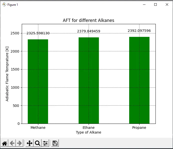
Effect of Number of Carbon Atoms(Methane, Ethane, Propane) on Adiabatic Flame Temprature

In the above CASE, the carbon atom of an alkane varied from 1 to 3 and the effect on AFT is studied. The combustion equation for the above class of hydrocarbons is given below :

METHANE :

`CH_4 + 2(O_2 + 3.76N_2) -> CO_2 + 2H_2O + 2(3.76N_2)`

ETHANE :

`C_2H_6 + 3.5(O_2 + 3.76N_2) -> 2CO_2 + 3H_2O + 3.5(3.76N_2)`

PROPANE :

`C_2H_8 + 5(O_2 + 3.76N_2) -> 3CO_2 + 4H_2O + 5(3.76N_2)`

Program for IVth CASE :

'''
AFT variation w.r.t number of carbon atoms chains
'''
import matplotlib.pyplot as plt
import cantera as ct

def h(T, coeff):

	R =8.314	 
	a1 =coeff[0]
	a2 =coeff[1]
	a3 =coeff[2]
	a4 =coeff[3]
	a5 =coeff[4]
	a6 =coeff[5]
	a7 =coeff[6]

	return (a1 + a2*(T/2) + a3*pow(T,2)/3 + a4*pow(T,3)/4 + a5*pow(T,4)/5 + a6/T )*R*T

ch4_coeffs_l  =[5.14987613E+00, -1.36709788E-02, 4.91800599E-05, -4.84743026E-08, 1.66693956E-11, -1.02466476E+04, -4.64130376E+00]
c2h6_coeffs_l =[4.29142492E+00, -5.50154270E-03, 5.99438288E-05, -7.08466285E-08, 2.68685771E-11, -1.15222055E+04, 2.66682316E+00]
c3h8_coeffs_l =[0.93355381E+00, 0.26424579E-01, 0.61059727E-05, -0.21977499E-07, 0.95149253E-11, -0.13958520E+05, 0.19201691E+02]
n2_coeffs_l   =[0.03298677E+02, 0.14082404E-02, -0.03963222E-04, 0.05641515E-07, -0.02444854E-10, -0.10208999E+04, 0.03950372E+02]
n2_coeffs_h   =[0.02926640E+02, 0.14879768E-02, -0.05684760E-05, 0.10097038E-09, -0.06753351E-13, -0.09227977E+04, 0.05980528E+02]
o2_coeffs_l   =[3.78245636E+00, -2.99673416E-03, 9.84730201E-06, -9.68129509E-09, 3.24372837E-12, -1.06394356E+03, 3.65767573E+00]
co2_coeffs_h  =[3.85746029E+00, 4.41437026E-03, -2.21481404E-06, 5.23490188E-10, -4.72084164E-14, -4.87591660E+04, 2.27163806E+00]
h2o_coeffs_h  =[3.03399249E+00, 2.17691804E-03, -1.64072518E-07, -9.70419870E-11, 1.68200992E-14, -3.00042971E+04, 4.96677010E+00]

# The standard reaction :- CxHy + (x + y/4)(O2 + 3.76N2) --> xCO2 + y/2H2O + (x + y/4)3.76N2


# Here we vary the value of n=1(Methane),2(Ethane),3(Propane), where x =2n and y =2n+2


# Methane_reaction	:CH4 + 2O2 + 2*3.76N2 = CO2 + 2H2O + 2*3.76 N2

def f_Methane(T):
	
	Tstp =298.15
	h_ch4_r =h(Tstp, ch4_coeffs_l)
	h_o2_r  =h(Tstp, o2_coeffs_l)
	h_n2_r  =h(Tstp, n2_coeffs_l)
	h_n2_p  =h(T, n2_coeffs_h)
	h_co2_p =h(T, co2_coeffs_h)
	h_h2o_p =h(T, h2o_coeffs_h)

	h_reactants =h_ch4_r + 2*h_o2_r + (2*3.76*h_n2_r)
	h_products  =h_co2_p + 2*h_h2o_p + (2*3.76*h_n2_p)

	return h_products - h_reactants

def fprime_Methane(T):
	return	(f_Methane(T + 1e-6) - f_Methane(T))/1e-6

# Etane_reaction : C2H6 + 3.5O2 + 3.5*3.76N2 --> 2CO2 + 3H2O + 3.5*3.76N2

def f_Ethane(T):
	
	Tstp =298.15
	h_c2h6_r =h(Tstp, c2h6_coeffs_l)
	h_o2_r =h(Tstp, o2_coeffs_l)
	h_n2_r =h(Tstp, n2_coeffs_l)
	h_n2_p =h(T, n2_coeffs_h)
	h_co2_p =h(T, co2_coeffs_h)
	h_h2o_p =h(T, h2o_coeffs_h)

	h_reactants =h_c2h6_r + 3.5*h_o2_r + (3.5*3.76*h_n2_r)
	h_products =2*h_co2_p + 3*h_h2o_p + (3.5*3.76*h_n2_p)

	return h_products - h_reactants

def fprime_Ethane(T):
	return	(f_Ethane(T + 1e-6) - f_Ethane(T))/1e-6


# Propane_reaction : C3H8 + 5O2 + 5*3.76N2 --> 3CO2 + 4H2O + 5*3.76N2

def f_Propane(T):

	Tstp =298.15
	h_c3h8_r =h(Tstp, c3h8_coeffs_l)
	h_o2_r =h(Tstp, o2_coeffs_l)
	h_n2_r =h(Tstp, n2_coeffs_l)
	h_n2_p =h(T, n2_coeffs_h)
	h_co2_p =h(T, co2_coeffs_h)
	h_h2o_p =h(T, h2o_coeffs_h)

	h_reactants =h_c3h8_r + 5*h_o2_r + (5*3.76*h_n2_r)
	h_products =3*h_co2_p + 4*h_h2o_p + (5*3.76*h_n2_p)

	return h_products - h_reactants

def fprime_Propane(T):
	return	(f_Propane(T + 1e-6) - f_Propane(T))/1e-6

T_Methane= 1500
T_Ethane= 1500
T_Propane= 1500
tol = 1e-3
alpha =1

T_aft =[]

while (abs(f_Methane(T_Methane))>tol):
	T_Methane = T_Methane - alpha*(f_Methane(T_Methane)/fprime_Methane(T_Methane))

T_aft.append(T_Methane)

while (abs(f_Ethane(T_Ethane))>tol):
	T_Ethane =T_Ethane -alpha*(f_Ethane(T_Ethane)/fprime_Ethane(T_Ethane)) 

T_aft.append(T_Ethane)

while (abs(f_Propane(T_Propane))>tol):
	T_Propane =T_Propane -alpha*(f_Propane(T_Propane)/fprime_Propane(T_Propane))

T_aft.append(T_Propane)

fuel = ['Methane','Ethane','Propane']
fuel_pos =[i for i, _ in enumerate(fuel)]

fig, ax =plt.subplots()
bars = ax.bar(fuel_pos, T_aft, width=0.4, color='green')
plt.xlabel('Type of Alkane')
plt.ylabel('Adiabatic Flame Temprature [K]')
plt.title("AFT for different Alkanes")
plt.xticks(fuel_pos, fuel)
plt.grid( linestyle=':', color='black')
plt.ylim((0, 2750))

for bar in bars:
	height =bar.get_height()
	ax.text(bar.get_x() + bar.get_width()/2., 1.05*height, '%f' % float(height), ha='center', va='bottom')


plt.show()			

Results:

Observation & Conclusion :-

• From above results we can conclude the aspected results the representation of Adiabatic Flame Temprature in the comparison of both python and cantera based software. We recieved the values from the NASA polynomial datasheet.
• On the second case we looked for the comparison of Flame Temprature and Heat Loss (in constant pressure chamber); the result is observed at the value of Heat_Loss at 50% of the maximum possible heat loss. The plot represents in between 0 to 1.
• On the third case we observed the bar graph representation of alkane, alkene and alkyenes of two carbon atom chains at 0% or no heat loss condition.The adiabatic flame temprature is varying as ethane is less than ethene and more lesser than that of ethyene.
• On the fourth case we observed the adiabatic flame temprature variation with respect to number of carbon atoms chains.The variation of the effect of carbon atoms from 1 to 3 on final temprature.