Week 3.5 - Deriving 4th order approximation of a 2nd order derivative using Taylor Table method

Derivation of central difference scheme, skewed right side and skewed left side difference scheme for fourth order approximation of second order derivativeby using Taylor Table Method of finite difference method

Aim:- The aim of this project is to derive central difference, skewed right difference and skewed left side difference difference scheme for fourth order approximation of second order derivative by using Taylor Table Method of finite difference method.

1. Central difference:

To derive central difference for fourth order approximation of second order derivative by using Taylor Table Method of finite difference method by using equation given below.

Second order derivatve of fourth order approximation by Central difference scheme :

`((del^2)f)/(del(x^2))`=af_i-2+bf_i-1+cf_i+df_i+1+ef_i+2

Taylor Table for central difference for fourth order approximation :

Stencil	f(i)	dxf’(i)	dx2f’’(i)	dx3f’’’(i)	dx4f’’’’(i)
afi-2	a	-2a	2a	-4a/3	2a/3
bfi-1	b	-b	b/2	-b/6	b/24
cfi	c	0	0	0	0
dfi+1	d	d	d/2	d/6	d/24
efi+2	e	2e	2e	4e/3	2e/3
	0	0	1	0	0

# MATLAB code to find the values of above coefficient :-

clear all
close all
clc

% Finding the coefficient for abve table
A = [1 1 1 1 1;-2 -1 0 1 2;2 1/2 0 1/2 2;-4/3 -1/6 0 1/6 4/3;2/3 1/24 0 1/24 2/3];
B = [0;0;1;0;0];
C = inv(A)*B;

C
C =

  -0.083333
   1.333333
  -2.500000
   1.333333
  -0.083333

Program for central differencing scheme :

function out =central_difference(x,dx)
  % Function = exp(x)*cos(x);
  %Analytical_derivative = exp(x)*cos(x)-exp(x)*sin(x);
  Second_order_derivative = -2*sin(x)*exp(x);
  % Numerical_derivative
  % Fourt_order_approximation
  central_difference = ((-0.08333*exp(x-2*dx)*cos(x-2*dx))+(1.33333*exp(x-1*dx)*cos(x-1*dx))-(2.50000*exp(x)*cos(x))+(1.33333*exp(x+1*dx)*cos(x+1*dx))-(0.08333*exp(x+2*dx)*cos(x+2*dx)))/(dx^2);
  out = abs(central_difference-Second_order_derivative);
endfunction

2. Skewed right side scheme

To derive central difference for fourth order approximation of second order derivative by using Taylor Table Method of finite difference method by using equation given below.

Second order derivatve of fourth order approximation by Skewed right side scheme :

`((del^2)f)/(del(x^2))`= af_i+bf_i+1+cf_i+2+df_i+3+ef_i+4

_{Taylor Table for central difference for fourth order approximation :}

Stencil	f(i)	dxf’(i)	dx2f’’(i)	dx3f’’’(i)	dx4f’’’’(i)
afi-2	a	0	0	0	0
bfi-1	b	b	b/2	b/6	b/24
cfi	c	2c	4c/2	8c/6	16c/24
dfi+1	d	3d	9d/2	27d/6	81d/24
efi+2	e	4e	16e/2	64e/6	256e/24
	0	0	1	0	0

# MATLAB code to find the value of above coefficient :

clear all
close all
clc

% Finding the coefficient for abve table
A = [1 1 1 1 1;0 1 2 3 4;0 1/2 4/2 9/2 16/2;0 1/6 8/6 27/6 64/6;0 1/24 16/24 81/24 256/24];
B = [0;0;1;0;0];
C = inv(A)*B;

ᩘ>> C
C =

   2.91667
  -8.66667
   9.50000
  -4.66667
   0.91667

>>

Program for skewed right side scheme :

function out = skewed_right_side_scheme(x,dx)
   % Function = exp(x)*cos(x);
  %Analytical_derivative = exp(x)*cos(x)-exp(x)*sin(x);
  Second_order_derivative = -2*sin(x)*exp(x);
  % Numerical_derivative
  % Fourt_order_approximation
  skewed_right_side_scheme= (2.91667*exp(x)*cos(x)-8.66667*exp(x+1*dx)*cos(x+1*dx)+9.50000*exp(x+2*dx)*cos(x+2*dx)-4.66667*exp(x+3*dx)*cos(x+3*dx)+0.91667*exp(x+4*dx)*cos(x+4*dx))/(dx^2);
  out = abs(skewed_right_side_scheme-Second_order_derivative);
endfunction

3. Skewed left side scheme :

To derive central difference for fourth order approximation of second order derivative by using Taylor Table Method of finite difference method by using equation given below.

Second order derivatve of fourth order approximation by Skewed left side scheme :

`((del^2)f)/(del(x^2))`= af_i+bf_i-1+cf_i-2+df_i-3+ef_i-4

Taylor Table for central difference for fourth order approximation :

Stencil	f(i)	dxf’(i)	dx2f’’(i)	dx3f’’’(i)	dx4f’’’’(i)
afi-2	a	0	0	0	0
bfi-1	b	-b	b/2	-b/6	b/24
cfi	c	-2c	2c	-8c/6	16c/24
dfi+1	d	-3d	9d/2	-27d/6	81d/24
efi+2	e	-4e	16e/2	-64e/6	256e/24
	0	0	1	0	0

# MATLAB code to find the value of above coefficient :

clear all
close all
clc

% Finding the coefficient for abve table
A = [1 1 1 1 1;0 -1 -2 -3 -4;0 1/2 4/2 9/2 16/2;0 -1/6 -8/6 -27/6 -64/6;0 1/24 16/24 81/24 256/24];
B = [0;0;1;0;0];
C = inv(A)*B;

>> C
C =

   2.91667
  -8.66667
   9.50000
  -4.66667
   0.91667

>>

Program for skewed left side scheme :

function out=skewed_left_side_scheme(x,dx)
    % Function = exp(x)*cos(x);
  %Analytical_derivative = exp(x)*cos(x)-exp(x)*sin(x);
  Second_order_derivative = -2*sin(x)*exp(x);
  % Numerical_derivative
  % Fourt_order_approximation
  skewed_left_side_scheme =(2.91667*exp(x)*cos(x)-8.66667*exp(x-dx)*cos(x-dx)+9.50000*exp(x-2*dx)*cos(x-2*dx)-4.66667*exp(x-3*dx)*cos(x-3*dx)+0.91667*exp(x-4*dx)*cos(x-4*dx))/(dx^2);
  out =abs(skewed_left_side_scheme-Second_order_derivative);
endfunction

Main Program :

clear all
close all
clc
% Input parameter
x= pi/3;
dx= linspace(pi/4,pi/4000,800);
% % Function = exp(x)8cos(x);
  %Analytical_derivative = exp(x)*cos(x)-exp(x)*sin(x);
  Second_order_derivative = -2*sin(x)*exp(x);
  % For_loop
  for i =1:length(dx)
    central_difference_errors(i) =central_difference(x,dx(i));
    skewed_right_side_scheme_errors(i) =skewed_right_side_scheme(x,dx(i));
    skewed_left_side_scheme_errors(i) =skewed_left_side_scheme(x,dx(i));
    
  endfor
  % plotting
  figure(1)
  loglog(dx,central_difference_errors,'r')
  hold on
  loglog(dx,skewed_right_side_scheme_errors,'g')
  hold on
  loglog(dx,skewed_left_side_scheme_errors,'b')
  xlabel('dx')
  ylabel('errors')
  legend('central_difference_errors','skewed_right_side_scheme_errors','skewed_left_side_scheme_errors')

Procedure followed :

1. Firstly according to the challenge we have to solve the analytical function for the fourth order approximation for three of the schemes namely central difference, skewed right side and skewed left side scheme.

2. The analytical function is needed to be solved for second order derivative as

Function = exp(x)*cos(x)
Analytical_derivative, f'(x) = exp(x)*cos(x)-exp(x)*sin(x)
Second_order_analytical_derivative, f''(x) = -2*sin(x)*exp(x)

3. So, now when we have solved the equation and the program has been written according to the sequence presented in the answer as firstly the function is solved for second order derivative and for fourth order approximation later the equation to be place in differencing are formed in taylor table form and the values of a, b, c, d, e are found respectively.

4.Later the values of coefficient of variables are placed in central difference form and placed in an function to find the out value by using the function 'abs' and the values are been called by the function in the main program.

5.Now, program has been written according to the sequence presented in the answer as firstly the function is solved for second order derivative and for fourth order approximation later the equation to be place in differencing are formed in taylor table form and the values of a, b, c, d, e are found respectively.

6.The values of coefficient of variables are placed in skewed right side difference form and placed in an function to find the out value by using the function 'abs' and the values are been called by the function in the main program.

7. Again program has been written according to the sequence presented in the answer as firstly the function is solved for second order derivative and for fourth order approximation later the equation to be place in differencing are formed in taylor table form and the values of a, b, c, d, e are found respectively.

8.The values of coefficient of variables are placed in skewed left side difference form and placed in an function to find the out value by using the function 'abs' and the values are been called by the function in the main program.

9.Now when all the values had been called in the main program , the values are called as by keeping the function name and '.m' extension file with the same name. The main program comprises the value of variables 'x' and 'dx' respectively.

10. The value of 'dx' is set by 'linspace' with specified range .

11. Now, at last we plot the following values by 'loglog' .

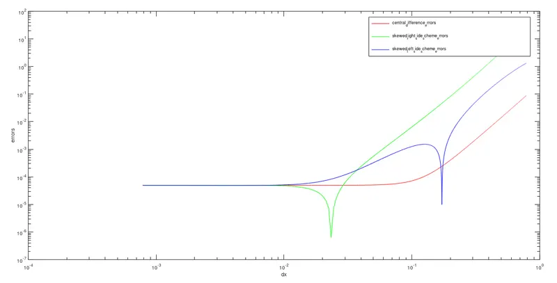
Final Result :

Conclusion :

There is a decreasing trend of the error with dx.After some point of time the values of dx is going horizontal .Basically the reason for this is because of low values of dx the round of errors are increasing.