Week 5.1 - Mid term project - Solving the steady and unsteady 2D heat conduction problem

Solving 2D steady state and Transient state heat conduction equation using MATLAB

This challenge is going to be quite hard and time consuming to finish. You have to solve the conduction equation using a transient equation using a transient solver and a steady state solver using iterative techniques (Jacobi,Gauss-Siedel,SOR).

1. Assume that domain is a unit square.
2. Assume nx =ny [Number of points along the x-direction is equal to the number of points along y-direction].
3. Boundary conditions for steady and transient case:-

• Top Boundary = 600 K
• Bottom Boundary = 900 K
• Left Boundary = 400 K
• Right Boundary = 800 K

Steps to be followed in order followed:

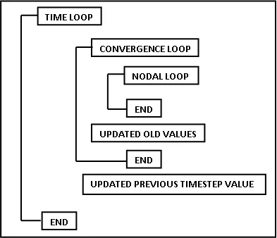
Steady-State Analysis & Transient State Analysis :

Solve the 2D heat conduction equation by using the point iterative technique that were taught in the class we will implement the following methods:

(1)Jacobi (2)Gauss-Siedel (3)Successive over relaxation

Our absolute error criteria are 1e-4.

Steady State Solution:

Discretizing the above equation

`(del^2 T) / (del x^2)` = (T_i-1,j - 2T_i,j + T_i+1,j) / `(delta x^2)`

`(del^2 T) / (del y^2)` = (T_i,j-1 - 2T_i,j + T_i,j+1) / `(delta y^2)`

As we consider nx = ny, `(delta x = delta y)`

Then rearranging the term, we get the equation like this

T_i,j = ¼ (T_i-1,j + T_i+1,j + T_i,j-1 + T_i,j+1)

MAIN PROGRAM (Steady State) :

%Solving the steady 2D heat conduction problem 
clear all
close all
clc  
%Input
L =1; %Length of domain and it is a square
% nx, ny no. of grid points
nx =30;
ny =nx;
x =linspace(0,1,nx);
y =linspace(0,1,ny);
dx =x(2)-x(1);
dy =y(2)-y(1);
error =9e9;
tol =1e-4;

%Define boundary condition
T_L =400;
T_T =600;
T_R =800;
T_B =900;
T =ones(nx,ny);
%Calculation of relaxation factor
%omega =2/(1+sin(pi*dx));
omega =1.2;

%Temprature at boundary
T(:,1)   =T_L;
T(:,end) =T_R;
T(end,:) =T_T;
T(1,:)   =T_B;

%Creating a copy of T
[X,Y] =meshgrid(x,y);
T_old =T;

%Jacobi_Method 
for iterative_solver =1
    tic;
    if iterative_solver ==1
       jacobi_iteration =1;
        while(error >tol)
            for i=2:nx-1
                for j=2:ny-1
                    T(i,j) =0.25*(T_old(i-1,j)+T_old(i+1,j)+T_old(i,j-1)+T_old(i,j+1));
                end
            end
            error =max(max(abs(T_old - T)));
            T_old =T;
            jacobi_iteration=jacobi_iteration+1;
        end
    end
    F =toc;
    %Plotting
    figure(1)
    [P,Q] =contourf(X,Y,T);
    clabel(P,Q);
    colormap(jet);
    colorbar;
    title_text =sprintf('Jacobi method,Iteration number = %d, computation time F =%fs',jacobi_iteration,F);
    title(title_text);
    xlabel('x axis');
    ylabel('y axis');
    fprintf('jacobi =%d/n', jacobi_iteration);
    pause(0.03);
end

%Gauss_siedel(GS) method
for iterative_solver = 2
    % update_values
L =1; %Length of domain and it is a square
% nx, ny no. of grid points
nx =30;
ny =nx;
x =linspace(0,1,nx);
y =linspace(0,1,ny);
dx =x(2)-x(1);
dy =y(2)-y(1);
error =9e9;
tol =1e-4;
%Define boundary condition
T_L =400;
T_T =600;
T_R =800;
T_B =900;
T =298*ones(nx,ny);
%Temprature at boundary
T(:,1) =T_L;
T(:,end) =T_R;
T(end,:) =T_T;
T(1,:) =T_B;

%Creating a copy of T
[X,Y] =meshgrid(x,y);
T_old =T;
tic;
if iterative_solver ==2
    gs_iteration =1;
    while(error >tol)
        for i =2:nx-1
            for j =2:ny-1
                T(i,j) =0.25*(T(i-1,j)+T_old(i+1,j)+T(i,j-1)+T_old(i,j+1));
            end
        end
        error =max(max(abs(T_old-T)));
        T_old =T;
        gs_iteration =gs_iteration + 1;
    end
    F =toc;
    %Plotting
    figure(2)
    [P,Q] =contourf(X,Y,T);
    clabel(P,Q);
    colormap(jet);
    colorbar;
    title_text =sprintf('Gauss Siedel, Iteration number =%d, computation time F =%fs',gs_iteration,F);
    title(title_text);
    xlabel('x axis');
    ylabel('y axis');
    fprintf('gs =%d/n',gs_iteration);
    pause(0.03);
end
end

   %SOR
   for iterative_solver =3
       %updated values
L =1; %Length of domain and it is a square
% nx, ny no. of grid points
nx =30;
ny =nx;
x =linspace(0,1,nx);
y =linspace(0,1,ny);
dx =x(2)-x(1);
dy =y(2)-y(1);
error =9e9;
tol =1e-4;
%Define boundary condition
T_L =400;
T_T =600;
T_R =800;
T_B =900;
T =ones(nx,ny);
%Calculation of relaxation factor
omega =2/(1+sin(pi*dx));
%Temprature at boundary
T(:,1) =T_L;
T(:,end) =T_R;
T(end,:) =T_T;
T(1,:) =T_B;
%Creating a copy of T
[X,Y] =meshgrid(x,y);
T_old =T;
k1=0.5*(dy^2/(dy^2+dx^2));
         k2=0.5*(dx^2/(dy^2+dx^2));
tic;
if iterative_solver ==3
    SOR_iteration =1;
    while(error >tol)
        for i=2:nx-1
            for j=2:ny-1
               % T(i,j) =((1-omega)*T_old(i,j)+(omega*0.25*(T(i-1,j)+T_old(i-1,j)+T_old(i+1,j)+T(i,j-1)+T_old(i,j+1))));
               
Tgauss(i,j)=k1*(T(i-1,j)+T_old(i+1,j))+k2*(T(i,j-1)+T_old(i,j+1));
              T(i,j)=(1-omega)*T_old(i,j)+omega*Tgauss(i,j);
            end
        end
        error =max(max(abs(T_old-T)));
        T_old =T;
        SOR_iteration =SOR_iteration+1;
    end
    F =toc;
    %Plotting
    figure(3)
    [P,Q] =contourf(X,Y,T);
    clabel(P,Q);
    colormap(jet);
    colorbar;
    title_text =sprintf('SOR,Iteration number =%d, computation time F =%fs',SOR_iteration,F);
    title(title_text);
    xlabel('x axis');
    ylabel('y axis');
    fprintf('SOR =%d/n',SOR_iteration);
    pause(0.03);
end
   end
   

OUTPUT :

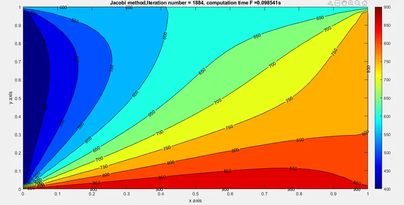
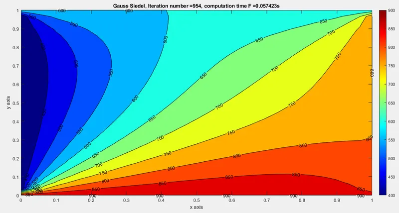
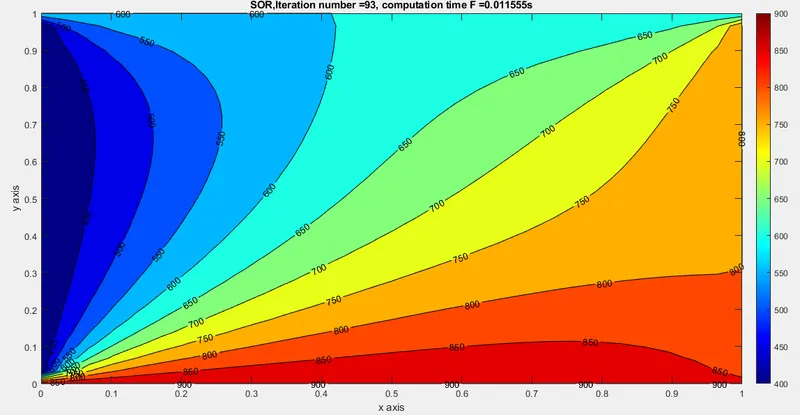
Transient or Unsteady State :

The Energy equation in 2D forms :

Assumptions:

1. No convection occurs.
2. No internal heat generation or dissipation.
3. Alpha being constant.

We discretizing the above equation:

Rearranging the terms we define two costants k1 and k2 :

k1 = `alpha (delta t) / (delta x^2)`

k2 = `alpha (delta t) / (delta y^2)`

Hence, `delta x = delta y`

Hence the equation is :

`(T^(n+1))_(i,j) = (T^(n))_(i,j) + k1((T^(n+1))_(i-1,j)-2(T^(n+1))_(i,j) + (T^(n+1))_(i+1,j)) + k2((T^(n+1))_(i,j-1)-2(T^(n+1))_(i,j) + (T^(n+1))_(i,j+1))`

`(T^(n+1))_(i,j) = ((T^(n))_(i,j) + k1(T_(i-1,j)) + k2(T_(i,j-1) + T_(i,j+1)))^(n+1)/(1 + 2k1 + 2k2)`

Hence, n denotes time indexnd (i,j) denotes the space index.

Main Program (Explicit):

%Solving the steady 2D transient unsteady state heat conduction problem
%explicit
clear all
close all
clc
% Inputs
L =1; %Length of domain and it is a square
% nx, ny no. of grid points
nx =51;
ny =nx;
x =linspace(0,1,nx);
y =linspace(0,1,ny);
dx =x(2)-x(1);
dy =y(2)-y(1);
error =9e9;
tol =1e-4;
dt =0.1;
alpha =1e-3; %Convective coefficient
t =5;
% CFL number
M =alpha*dt/(dx^2);
%Define boundary conditions
T_L =400;
T_T =600;
T_R =800;
T_B =900;
T =298*ones(nx,ny);
%Temprature at boundary
T(:,1) =T_L;
T(:,end) =T_R;
T(end,:) =T_B;
T(1,:) =T_T;

%Average Temprature at the corner matrix
T(1,1) =(T_T + T_L)/2;
T(1,end) =(T_T + T_R)/2;
T(end,1) =(T_L + T_B)/2;
T(end,end) =(T_R + T_B)/2;

%Calculation of temprature distribution explicitly using iterative solvers
k1 =(alpha*dt)/(dx^2);
k2 =(alpha*dt)/(dy^2);

%creating a copy of T
[X,Y] =meshgrid(x,y);
Told =T;
nt =t/dt;

%2D transient unsteady state heat conduction equation in explicit method
iterative_solver =1;
tic;
iterations =1;
for v= 1:nt
    if iterative_solver == 1
        error =100;
        while(error >tol)
            for i=2:nx-1
                for j=2:ny-1
                    term1 =Told(i,j);
                    term2 =k1*(Told(i+1,j)-2*Told(i,j)+Told(i-1,j));
                    term3 =k2*(Told(i,j+1)-2*Told(i,j)+Told(i,j-1));
                    T(i,j) =term1 + term2 + term3;
                end
            end
            error =max(abs(Told-T));
            Told =T;
            iterations =iterations+1;
        end
    end
    time =toc;
    %Plotting
    figure(1)
    [P,Q] =contourf(X,Y,T);
    clabel(P,Q,'fontsize',12);
    colormap(jet);
    colorbar;
    title_text= sprintf('Explicit method",Iteration number=%d,computation time=%fs, M=%f',iterations,time,M);
    title(title_text);
    xlabel =('xaxis');
    ylabel =('yaxis');
    pause(0.03);
end

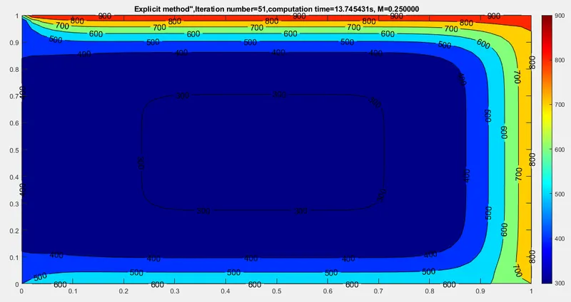
Output :

Program (Implicit Method):

%Solving the steady 2D transient unsteady state heat conduction problem
%explicit
clear all
close all
clc
% Inputs
L =1; %Length of domain and it is a square
% nx, ny no. of grid points
nx =20;
ny =nx;
x =linspace(0,1,nx);
y =linspace(0,1,ny);
dx =x(2)-x(1);
dy =y(2)-y(1);
error =9e9;
tol =1e-4;
dt =0.1;
alpha =1e-3; %Convective coefficient
t =5;
% CFL number
M =alpha*dt/(dx^2);
%Define boundary conditions
T_L =400;
T_T =600;
T_R =800;
T_B =900;
T =298*ones(nx,ny);
%Temprature at boundary
T(:,1) =T_L;
T(:,end) =T_R;
T(end,:) =T_B;
T(1,:) =T_T;

%Average Temprature at the corner matrix
T(1,1) =(T_T + T_L)/2;
T(1,end) =(T_T + T_R)/2;
T(end,1) =(T_L + T_B)/2;
T(end,end) =(T_R + T_B)/2;

%Calculation of temprature distribution explicitly using iterative solvers
k1 =(alpha*dt)/(dx^2);
k2 =(alpha*dt)/(dy^2);
nt =t/dt;

%creating a copy of T
[X,Y] =meshgrid(x,y);
Told =T;
T_prev_dt =Told;

%Calculating 2D heat conduction equation(implicitly)
%Jacobi method
nt =t/dt;
iterative_solver =1;
tic;
jacobi_iteration =1;
for v=1:nt
    if iterative_solver == 1
        term1 =(1+2*k1+2*k2)^(-1);
        term2 =k1*term1;
        term3 =k2*term2;
        error =100;
        while(error >tol)
            for i=2:nx-1
                for j=2:ny-1
                    H =(Told(i-1,j)+Told(i+1,j));
                    V =(Told(i,j-1)+Told(i,j+1));
                    T(i,j) =(T_prev_dt(i,j)*term1)+(H*term2)+(V*term3);
                end
            end
            error =max(abs(Told-T));
            Told =T;
            jacobi_iteration =jacobi_iteration+1;
        end
        F =toc;
        %Plotting
        figure(1)
        [P,Q] =contourf(X,Y,T);
        clabel(P,Q,'fontsize',12);
        colormap(jet);
        colorbar;
        title_text =sprintf('Jacobi metod,Iteration number =%d,computation time F =%fs,M =%f',jacobi_iteration,F,M);
        title(title_text);
        xlabel('x axis');
        ylabel('y axis');
        pause(0.03);
    end
end

%Gauss Siedel method
%update value
%Input
L =1; %Length of domain and it is a square
% nx, ny no. of grid points
nx =20;
ny =nx;
x =linspace(0,1,nx);
y =linspace(0,1,ny);
dx =x(2)-x(1);
dy =y(2)-y(1);
error =9e9;
tol =1e-4;
dt =0.1;
alpha =1e-3; %Convective coefficient
t =5;
% CFL number
M =alpha*dt/(dx^2);
%Define boundary conditions
T_L =400;
T_T =600;
T_R =800;
T_B =900;
T =298*ones(nx,ny);
%Temprature at boundary
T(:,1) =T_L;
T(:,end) =T_R;
T(end,:) =T_B;
T(1,:) =T_T;

%Average Temprature at the corner matrix
T(1,1) =(T_T + T_L)/2;
T(1,end) =(T_T + T_R)/2;
T(end,1) =(T_L + T_B)/2;
T(end,end) =(T_R + T_B)/2;

%Calculation of temprature distribution explicitly using iterative solvers
k1 =(alpha*dt)/(dx^2);
k2 =(alpha*dt)/(dy^2);
nt =t/dt;

%creating a copy of T
[X,Y] =meshgrid(x,y);
Told =T;
T_prev_dt =Told;
iterative_solver =2;
tic;
gs_iteration =1;
for w =1:nt
    if iterative_solver == 2
          term1 =(1+2*k1+2*k2)^(-1);
        term2 =k1*term1;
        term3 =k2*term2;
        error =100;
        while(error >tol)
            for i=2:nx-1
                for j=2:ny-1
                    H =(Told(i-1,j)+Told(i+1,j));
                    V =(Told(i,j-1)+Told(i,j+1));
                    T(i,j) =(T_prev_dt(i,j)*term1)+(H*term2)+(V*term3);
                end
            end
            error =max(abs(Told-T));
            Told =T;
            gs_iteration =gs_iteration+1;
        end
        T_prev_dt =T;
        F =toc;
        %Plotting
        figure(2)
        [P,Q] =contourf(X,Y,T);
        clabel(P,Q);
        colormap(jet);
        colorbar;
        title_text =sprintf('Gauss Siedel,Iteration number F=%d,computation time F=%fs,M=%f',gs_iteration,F,M);
        title(title_text);
        xlabel('x axis');
        ylabel('y axis');
        pause(0.03);
    end
end

%SOR method
%update values
iterative_solver =3;
%Inputs
L =1; %Length of domain and it is a square
% nx, ny no. of grid points
nx =20;
ny =nx;
x =linspace(0,1,nx);
y =linspace(0,1,ny);
dx =x(2)-x(1);
dy =y(2)-y(1);
error =9e9;
tol =1e-4;
dt =0.1;
alpha =1e-3; %Convective coefficient
t =5;
% CFL number
M =alpha*dt/(dx^2);
%Calculation of relaxation number
omega =1.2;

%Define boundary conditions
T_L =400;
T_T =600;
T_R =800;
T_B =900;
T =ones(nx,ny);
%Temprature at boundary
T(:,1) =T_L;
T(:,end) =T_R;
T(end,:) =T_B;
T(1,:) =T_T;

%Average Temprature at the corner matrix
T(1,1) =(T_T + T_L)/2;
T(1,end) =(T_T + T_R)/2;
T(end,1) =(T_L + T_B)/2;
T(end,end) =(T_R + T_B)/2;

%Calculation of temprature distribution explicitly using iterative solvers
k1 =(alpha*dt)/(dx^2);
k2 =(alpha*dt)/(dy^2);

%creating a copy of T
[X,Y] =meshgrid(x,y);
Told =T;
T_prev_dt =Told;
tic;
SOR_iteration =1;
for z=1:nt
    if iterative_solver == 3
        term1 =(1+2*k1+2*k2)^(-1);
        term2 =k1*term1;
        term3 =k2*term2;
        error =100;
        while(error >tol)
            for i=2:nx-1
                for j=2:ny-1
                    H =(omega*Told(i-1,j)+(1-omega)*Told(i-1,j)+Told(i+1,j));
                    V =(omega*Told(i,j-1)+(1-omega)*Told(i,j-1)+Told(i,j+1));
                    T(i,j) =(T_prev_dt(i,j)*term1)+(H*term2)+(V*term3);
                end
            end
            error =max(abs(Told - T));
            Told =T;
            SOR_iteration =SOR_iteration+1;
        end
        T_prev_dt =T;
        F =toc;
        %Plotting
        figure(3)
        [P,Q] =contourf(X,Y,T);
        clabel(P,Q);
        colormap(jet);
        colorbar;
        title_text =sprintf('SOR method, Iteration number =%d,computation time F=%fs,M =%f',SOR_iteration,F,M);
        title(title_text);
        xlabel('x axis');
        ylabel('y axis');
        pause(0.03);
    end
end

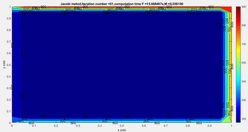
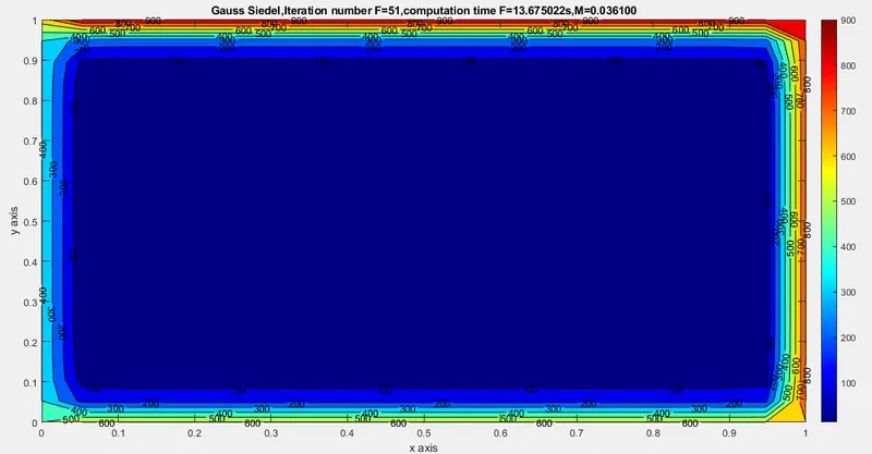
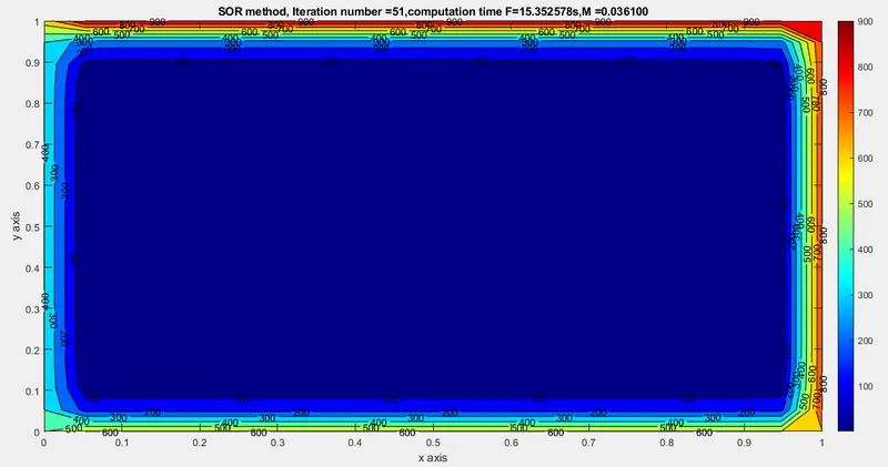
Output :

Conclusion:

From the above plots, it can be confirmed that the SOR takes minimum time for converging solution with fewer iteration and minimum error values when compared with Jacobi and Gauss Seidel method.

The transient state requires more computational time than the steady state. It takes more time to reach steady-state condition. In implicit method , it takes more time for converging compared to the explicit method. When it comes to CFL number<0.25 we can use an explicit method.

For steady state equation compared to Jacobi and Gauss Seidel method, the solver SOR is very efficient because it takes less convergence with fewer iterations for giving steady state solutions.

In transient sate explicit method has the least convergence time but it can be used when CFL number less than0.25, Jacobi has less convergence time and gauss seidel but overall SOR, is very efficient with fewer iterations and less convergence time.