Week 7 - Simulation of a 1D Super-sonic nozzle flow simulation using Macormack Method
Simulation of a 1D Super-sonic nozzle flow simulation using Macormack Method
Objective :
To solve the system of equations for quassi steady convergent-divergent 1D-ozzle using MacCormack method applying both Conservative and Non-Conservative form of equation.
Flow Field :
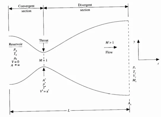
- Consider an steady, isentropic flow
- Since the flow is quassi 1D flow, the properties vary along the x-axis.
- Based on Mach Number mentioned, the flow is:
Inlet = Subsonic
Outlet = Supersonic
Non-Conservative Form :
Governing Equation



Initial Condition at t=0
rho =1-0.3146*x;
T =1-0.2314*x;
V =(0.1 + 1.09*x).*T.^(1/2);
A =1+2.2*(x - 1.5).^2;
Boundary Condition
At Subsonic Flow
rho=1
T=1
At supersonic flow
Boundary Condition
V(n) = 2*V(n-1) -V(n-2);
rho(n) = 2*rho(n-1) -rho(n-2);
T(n) = 2*T(n-1) -T(n-2);
Conservative Form :
Governing Equation
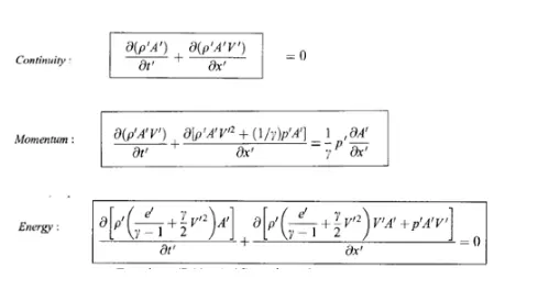
By defining solution vector U, flux vector U, flux vector F and source term J, we can rewrite the equation as below:
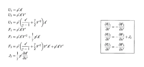
Further simplification to eliminate the dependant variable gives us
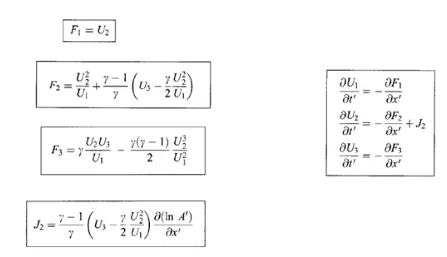
Initial Condition at t=0
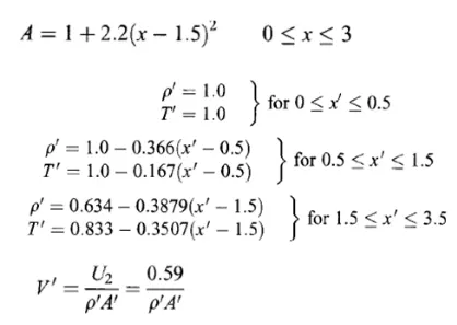
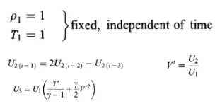
Boundary Condition
At subsonic flow,
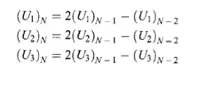
At supersonic flow,
Calculation of time step :
Using the Courant Friedrichs Lowry conditions
dt =C*dx/(a+v);
Considering non-dimensional form, we can rewrite it as
dt =C*dx/(T^(1/2)+V);
For a stable solution C<1. For this case assume C=0.5.
The time step for the given system is determined dt at all grid point and calculating the minimum value
dt =min(dt1,dt2,......dtN).
Program algorithm- MacCormack Method
- Calculate the initial conditions.
- Determine the predictor time derivative terms for continuity, momentum and energy conditions using Forward difference scheme for space derivative.
- Update the solution.
- Determine the corrector time derivative terms by using BDS.
- Calulate the average time derivative.
- Update the final solution.
- Calculate the inlet and outlet boundary conditions.
- Repeat the process for given timesteps nt.
Main Program :
clear all
close all
clc

n =31;
x =linspace(0,3,n);
dx =x(2)-x(1);
n1 =61;
x1 =linspace(0,3,n1);
dx1 =x(2)-x(1);

nt =1400;

%Area
A  =1+2.2*(x - 1.5).^2;
A1 =1+2.2*(x1 - 1.5).^2;

%Non-Conservation Solution n=31
[rho_nc, V_nc, T_nc, M_nc, P_nc] =Nonconservative(A,nt,n,dx,x);

%Non-Conservative solution for n=61
[rho_nc1, V_nc1, T_nc1, M_nc1, P_nc1] =Nonconservative1(A1,nt,n1,dx1,x1);

%Conservative Solution
[rho_c, V_c, T_c, M_c, P_c, rho_15, T_15, V_15] =conservative(A,nt,n,dx,x)

figure(1)
plot(x,rho_c)
hold on
plot(x,rho_nc,'*')
xlabel('Domain x/L')
ylabel('Density ratio rho/rho_0')
legend('Conservative','Non-Conservative')

figure(2)
plot(x,V_c)
hold on
plot(x,V_nc,'*')
xlabel('Domain x/L')
ylabel('Velocity ratio V/a_0')
legend('Conservative','Non-Conservative')

figure(3)
plot(x,T_c)
hold on
plot(x,T_nc,'*')
xlabel('Domain x/L')
ylabel('Temprature ratio T/T_0')
legend('Conservative','Non-Conservative')

figure(4)
plot(x,P_c)
hold on
plot(x,P_nc,'*')
xlabel('Domain x/L')
ylabel('Pressure ratio P/P_0')
legend('Conservative','Non-Conservative')

figure(5)
plot(x,M_c)
hold on
plot(x,M_nc,'*')
xlabel('Domain x/L')
ylabel('MAch Number')
legend('Conservative','Non-Conservative')

figure(6)
subplot(3,1,1)
plot([1:1400], rho_15)
xlabel('Time step t')
ylabel('Density ratio rho/rho_0')
title('Variation of properties at i=15 with timestep')

subplot(3,1,2)
plot([1:1400],T_15)
xlabel('Time step T')
ylabel('Temprature ratio T/T_0')

subplot(3,1,3)
plot([1:1400],V_15)
xlabel('Time step T')
ylabel('Velocity ratio V/a_0')

figure(7)
plot(x1,rho_nc1)
hold on
plot(x,rho_nc,'*')
xlabel('Domain x/L')
ylabel('Density ratio rho/rho_0')
legend('Solution for n=61','Solution for n=31')
title('Grid Independence test')

figure(8)
plot(x,rho_nc.*V_nc.*A,'r')
hold on
plot(x,rho_c.*V_c.*A,'g')
hold on
plot(x,0.579*ones(size(x)),'b')
xlabel('Domain x/L')
ylabel('Mass flow rho*V*A')
legend('Non-Conservative','Conservative','Analytical-Solution')
title('Steady state mass flow rate variation')
Function for Non-Conservative for n=31 :
%Function for nonconservative form of equation
function[rho, V, T, M, P] =Nonconservative(A,nt,n,dx,x)

%Initial Condition at t=0
rho =1-0.3146*x;
T =1-0.2314*x;
V =(0.1 + 1.09*x).*T.^(1/2);

%boundary condition
V(n)   = 2*V(n-1) -V(n-2);
rho(n) = 2*rho(n-1) -rho(n-2);
T(n)   = 2*T(n-1) -T(n-2);

%Calculation of timestep
C=0.5;
for i=1:n
    timestep(i) =C*dx/(T(i)^(1/2)+V(i));
end
dt =min(timestep);

gamma =1.4;

%Timeloop
for t=1:nt

    %Store initial values
    rho_initial =rho;
    V_initial =V;
    T_initial =T;

    %MacCormack  method for time t
    for i=2:n-1
        drhodx =(rho(i+1) -rho(i))/dx;
        dVdx =(V(i+1) -V(i))/dx;
        dlnAdx =(log(A(i+1))-log(A(i)))/dx;
        dTdx =(T(i+1)-T(i))/dx;

        %Calculate predictor time derivative
        drhodt_p =-rho(i)*dVdx -rho(i)*V(i)*dlnAdx -V(i)*drhodx;
        dVdt_p = -V(i)*dVdx-(1/gamma)*(dTdx+(T(i)/rho(i))*drhodx);
        dTdt_p = -V(i)*dTdx -(gamma-1)*T(i)*(dVdx +V(i)*dlnAdx);

        %Solution updation
        rho(i) =rho(i) + drhodt_p*dt;
         V(i) =V(i) + dVdt_p*dt;
         T(i) =T(i) + dTdt_p*dt;

        %BDS
        drhodx_c = (rho(i)-rho(i-1))/dx;
        dVdx_c = (V(i) -V(i-1))/dx;
        dlnAdx_c =(log(A(i)) -log(A(i-1)))/dx;
        dTdx_c =(T(i) -T(i-1))/dx;

        %Calculate corrector time derivative
        drhodt_c =-rho(i)*dVdx_c -rho(i)*V(i)*dlnAdx_c -V(i)*drhodx_c;
        dVdt_c = -V(i)*dVdx_c-(1/gamma)*(dTdx_c+(T(i)/rho(i))*drhodx_c);
        dTdt_c = -V(i)*dTdx_c -(gamma-1)*T(i)*(dVdx_c +V(i)*dlnAdx_c);

        %Calculate average time derivative
        drhodt_avg =0.5*(drhodt_p + drhodt_c);
        dVdt_avg =0.5*(dVdt_p + dVdt_c);
        dTdt_avg =0.5*(dTdt_p + dTdt_c);

        %Calculate Final Solution
        rho(i) =rho_initial(i) + drhodt_avg*dt;
        V(i)   =V_initial(i) + dVdt_avg*dt;
        T(i)   =T_initial(i) + dTdt_avg*dt;
    end
        M =V./T.^(1/2);
        P =rho.*T;

    end
end
Function for Non-Conservative for n=61 :
%Function for nonconservative form of equation
function[rho, V, T, M, P] =Nonconservative1(A1,nt,n1,dx1,x1)

%Initial Condition at t=0
rho =1-0.3146*x1;
T =1-0.2314*x1;
V =(0.1 + 1.09*x1).*T.^(1/2);

%boundary condition
V(n1)   = 2*V(n1-1) -V(n1-2);
rho(n1) = 2*rho(n1-1) -rho(n1-2);
T(n1)   = 2*T(n1-1) -T(n1-2);

%Calculation of timestep
C=0.5;
for i=1:n1
    timestep(i) =C*dx1/(T(i)^(1/2)+V(i));
end
dt =min(timestep);

gamma =1.4;

%Timeloop
for t=1:nt

    %Store initial values
    rho_initial =rho;
    V_initial =V;
    T_initial =T;

    %MacCormack  method for time t
    for i=2:n1-1
        drhodx =(rho(i+1) -rho(i))/dx1;
        dVdx =(V(i+1) -V(i))/dx1;
        dlnAdx =(log(A1(i+1))-log(A1(i)))/dx1;
        dTdx =(T(i+1)-T(i))/dx1;

        %Calculate predictor time derivative
        drhodt_p =-rho(i)*dVdx -rho(i)*V(i)*dlnAdx -V(i)*drhodx;
        dVdt_p = -V(i)*dVdx-(1/gamma)*(dTdx+(T(i)/rho(i))*drhodx);
        dTdt_p = -V(i)*dTdx -(gamma-1)*T(i)*(dVdx +V(i)*dlnAdx);

        %Solution updation
        rho(i) =rho(i) + drhodt_p*dt;
        T(i) =T(i) + dTdt_p*dt;
        V(i) =V(i) + dVdt_p*dt;

        %BDS
        drhodx_c = (rho(i)-rho(i-1))/dx1;
        dVdx_c = (V(i) -V(i-1))/dx1;
        dlnAdx_c =(log(A1(i)) -log(A1(i-1)))/dx1;
        dTdx_c =(T(i) -T(i-1))/dx1;

        %Calculate corrector time derivative
        drhodt_c =-rho(i)*dVdx_c -rho(i)*V(i)*dlnAdx_c -V(i)*drhodx_c;
        dVdt_c = -V(i)*dVdx_c-(1/gamma)*(dTdx_c+(T(i)/rho(i))*drhodx_c);
        dTdt_c = -V(i)*dTdx_c -(gamma-1)*T(i)*(dVdx_c +V(i)*dlnAdx_c);

        %Calculate average time derivative
        drhodt_avg =0.5*(drhodt_p + drhodt_c);
        dVdt_avg =0.5*(dVdt_p + dVdt_c);
        dTdt_avg =0.5*(dTdt_p + dTdt_c);

        %Calculate Final Solution
        rho(i) =rho_initial(i) + drhodt_avg*dt;
        V(i)   =V_initial(i) + dVdt_avg*dt;
        T(i)   =T_initial(i) + dTdt_avg*dt;
    end
        M =V./T.^(1/2);
        P =rho.*T;

    end
end
Function for Conservative Form :
function[rho, V, T, M, P, rho_15, T_15, V_15] =conservative(A,nt,n,dx,x)

gamma =1.4;
%Initial Condition
for k=1:n
    if x(k)>=0 && x(k)<=0.5
        rho(k)=1;
        T(k)=1;
    elseif x(k)>0.5 && x(k)<=1.5
        rho(k) =1-0.366*(x(k)-0.5);
        T(k) =1-0.167*(x(k)-0.5);
    elseif x(k)>1.5 && x(k)<=3.5
        rho(k) =0.634 -0.3879*(x(k)-1.5);
        T(k) =0.833 -0.3507*(x(k)-1.5);
    end
end
V =0.59./(rho.*A);

U1 =rho.*A;
U2 =rho.*A.*V;
U3 =rho.*((T/(gamma-1))+(gamma/2).*V.^2).*A;

%Calculation of time step
C =0.5;
for i=2:n-1
    timestep(i-1) =C*dx/(T(i)^(1/2)+V(i));
end
dt =min(timestep);

%Timeloop
for t= 1:nt
    %Store initial value
    U1_initial =U1;
    U2_initial =U2;
    U3_initial =U3;

    F1_p =U2;
    F2_p =(U2.^2./U1) + ((gamma-1)/gamma)*(U3-(gamma/2)*(U2.^2./U1));
    F3_p =(gamma*U2.*U3./U1)-((gamma*(gamma-1)/2)*U2.^3./U1.^2);

    %MacCormack Method for time t
    for i=2:n-1

        %Calculate predictor time derivative
        dU1dt_p(i)= -(F1_p(i+1) -F1_p(i))/dx;
        J2_p(i)= (1/gamma)*rho(i).*T(i).*(A(i+1) -A(i))/dx;
        dU2dt_p(i)= -((F2_p(i+1) -F2_p(i))/dx)+J2_p(i);
        dU3dt_p(i)= -(F3_p(i+1) -F3_p(i))/dx;

        %Calculate updated solution
        U1(i)= U1(i) +dU1dt_p(i)*dt;
        U2(i)= U2(i) +dU2dt_p(i)*dt;
        U3(i)= U3(i) +dU3dt_p(i)*dt;
    end

    %Predictor loop end
    rho= U1./A;
    T= (gamma-1)*(U3./U1 -(gamma/2)*(U2./U1).^2);
    F1_c= U2;
    F2_c= (U2.^2./U1)+((gamma-1)/gamma)*(U3-(gamma/2)*(U2.^2./U1));
    F3_c =(gamma*U2.*U3./U1)-((gamma*(gamma-1)/2)*U2.^3./U1.^2);

    for i=2:n-1

        %Calculator corrector time derivative
        dU1dt_c(i)= -(F1_c(i) -F1_c(i-1))/dx;
        J2_c(i)= (1/gamma)*rho(i).*T(i).*(A(i)-A(i-1))/dx;
        dU2dt_c(i)= -((F2_c(i) -F2_c(i-1))/dx)+J2_c(i);
        dU3dt_c(i)= -(F3_c(i)-F3_c(i-1))/dx;

        %Calculate avg time derivative
        dU1dt_avg(i)= 0.5*(dU1dt_c(i) +dU1dt_p(i));
        dU2dt_avg(i)= 0.5*(dU2dt_c(i) +dU2dt_p(i));
        dU3dt_avg(i)= 0.5*(dU3dt_c(i) +dU3dt_p(i));

        U1(i)= U1_initial(i)+dU1dt_avg(i)*dt;
        U2(i)= U2_initial(i)+dU2dt_avg(i)*dt;
        U3(i)= U3_initial(i)+dU3dt_avg(i)*dt;
    end

    %Boundary Condition at inlet
    U1(1)= rho(1)*A(1);
    U2(1)= 2*U2(2)-U2(3);
    V(1)= U2(1)/(rho(1)*A(1));

    %Boundary Condition at Outlet
    U1(n)= 2*U1(n-1) -U1(n-2);
    U2(n)= 2*U2(n-1) -U2(n-2);
    U3(n)= 2*U3(n-1) -U3(n-2);

    rho= U1./A;
    V = U2./U1;
    T =(gamma-1)*((U3./U1)-(gamma/2)*V.^2);
    M =V./T.^(1/2);
    P =rho.*T;

    %Variation of primitive variable with timestep at i=15(A=1)
    rho_15(t) =rho(15);
    T_15(t) =T(15);
    V_15(t) =V(15);
end
%Timeloop end
end
%Function loop end
Results :
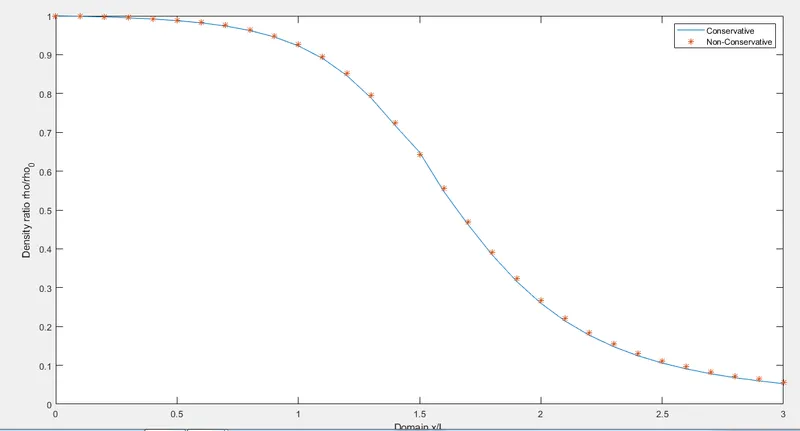
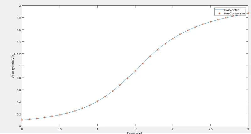
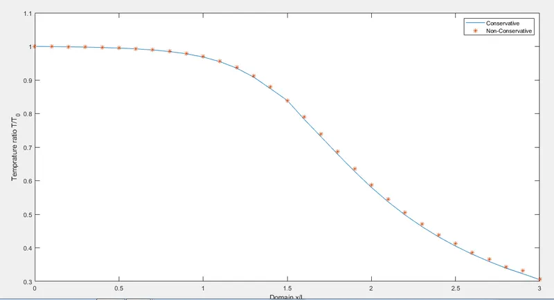
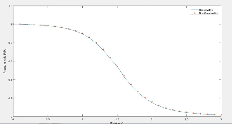
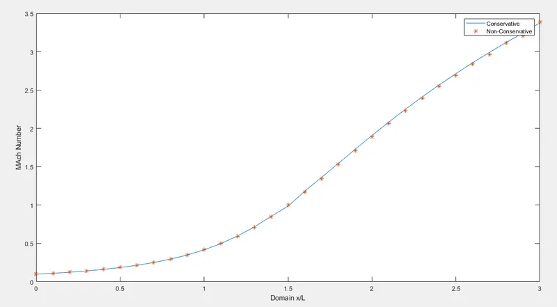
- Plot of properties for conservative and non-conservative form
- Density
- Velocity
- Temprature
- Pressure
- Mach Number
- Variation of properties with time at throat
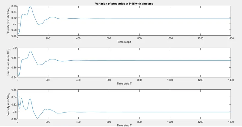
The properties oscillate at the lower time steps and attain steady state after approximately 450 timesteps. That is the solution converges at timestep nt =450.
- Grid Independence Test
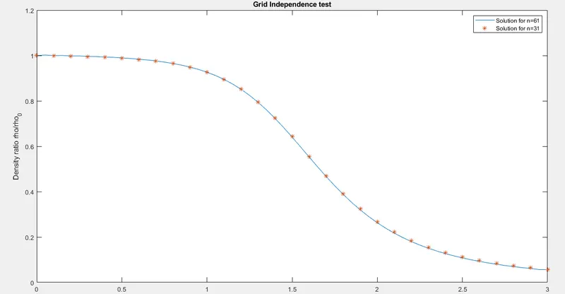
A comparison plot of the density ratio for grid point n=31 and n=61 show that the results do not vary with the increase in number of grid points/decrease in grid size.
In other words the solution obtained n=31 is grid independent solution.
- Steady State Mass Flow Variations :
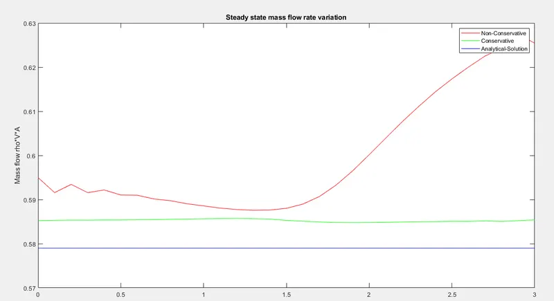
It is observed that the steady state mass flow is less significant in the case of conservative form of solution as the flux variable U2=rho.V.A (mass flow) is used to compute the solution.
Since, non-conservative solution uses primitive variable rho,V & T. Hence, the variation in the flux parameter is significant.
Conclusion :
- Programming Convenience
- Non-Conservative form is convenient as primitive variables are only to be defined.
- Application to complex problems
- In problems with the non-continous functions or multiple oscillations in properties across the domain non-conservative solution may blow up.
- Conservative solution being dependent on flux variables absorb the oscillation of primitive variables and giving stable , converging solution.