Week 3.5 - Deriving 4th order approximation of a 2nd order derivative using Taylor Table method

Quuestion :

1. Central difference

2. Skewed right-sided difference

3. Skewed left-sided difference

After deriving these schemes, prove that your skewed schemes are fourth-order accurate i.e the thumb rule given in HINT (ii). 

Once you have done this, write a program in Matlab to evaluate the second-order derivative of the analytical function exp(x)*cos(x) and compare it with the 3 numerical approximations that you have derived.

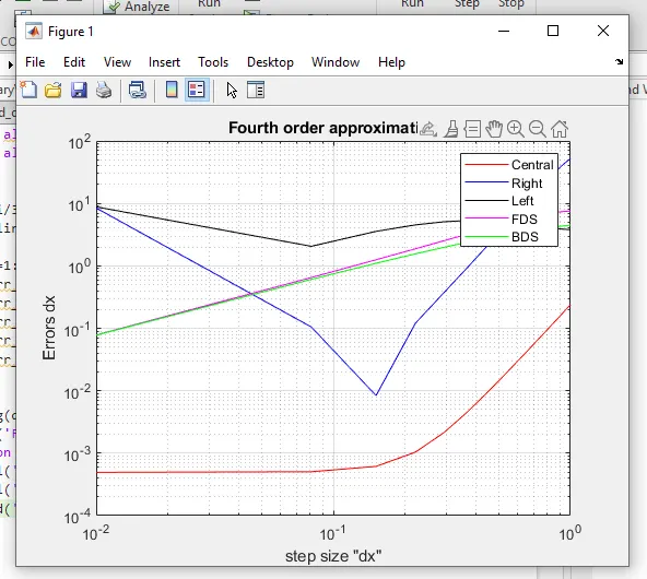
Provide a plot that compares the absolute error between the above-mentioned schemes

In your own words, describe why a skewed scheme is useful? What can a skewed scheme do that a CD scheme cannot?

HINT :

i) The order of accuracy P = Number of nodes in the stencil N - order of derivative Q + 1 for symmetric/central schemes

ii) The order of accuracy P = Number of nodes in the stencil N - order of derivative Q   for one-sided/skewed schemes 

iii) Solve the system of equations using the matrix inversion method in Matlab to obtain the taylor table coefficients and use them directly in the numerical approximation statements to avoid input errors. 

 Answer :

1. Centrial Diffrence Scheme:

The Centrial Diffrence Scheme uses a symmetric stencil. In this case, we want a fourth-order accurate approximation for the second-order derivative, so N - Q + 1 = 4, which implies N = 5.

Let's assume a function f(x), and we want to find its second-order derivative at a point x0.

The stencil with 5 nodes centered at x0 is: 

x0 - 2h, x0 - h, x0, x0 + h, x0 + 2h

Using Taylor series expansion, you can write down the approximations for the function values at these points and derive the central difference formula for the second-order derivative.

2. Skewed Right-sided Difference Scheme:

In this case, we want a fourth-order accurate approximation for the second-order derivative, so N - Q = 4, which implies N = 6.

The stencil with 6 nodes is:

x0, x0 + h, x0 + 2h, x0 + 3h, x0 + 4h, x0 + 5h

Again, using Taylor series expansion, you can write down the approximations for the function values at these points and derive the skewed right-sided difference formula for the second-order derivative.

3. Skewed Left-sided Difference Scheme:

This is similar to the skewed right-sided difference but with nodes to the left of x0.

In this case, we want a fourth-order accurate approximation for the second-order derivative, so N - Q = 4, which implies N = 6.

The stencil with 6 nodes is: 

x0 - 5h, x0 - 4h, x0 - 3h, x0 - 2h, x0 - h, x0

Using Taylor series expansion, you can write down the approximations for the function values at these points and derive the skewed left-sided difference formula for the second-order derivative.

Why a Skewed Scheme is Useful:

A skewed scheme is useful because it allows you to approximate derivatives in cases where you may not have symmetric data points or where you want to emphasize information from one side of the point of interest more than the other.

For example, in fluid dynamics or heat conduction problems, information may be moving predominantly in one direction, and a skewed scheme can capture this behavior more accurately. It can also be useful when you have irregularly spaced data points or when you want to avoid including points that are not relevant to the local behavior of the function.

A skewed scheme can do what a central difference (CD) scheme cannot by allowing you to tailor the stencil to your specific problem. CD schemes use symmetric stencils and may not be suitable when you need to account for directional or asymmetric behavior. Skewed schemes provide greater flexibility in choosing the stencil points, making them more versatile in various numerical applications.

Matlab main programe

clear all
close all
clc
 
x = pi/3;
dx = linspace(0.01,1,15);
 
for i=1:length(dx)
err_secondOrderForward(i) = second_order_forward_approx(x,dx(i));
err_secondOrder(i) = second_order_approx(x,dx(i));
err_centralDiff(i) = fourth_central(x,dx(i));
err_skewedRight(i) = fourth_skewed_right(x,dx(i));
err_skewedLeft(i) = fourth_skewed_left(x,dx(i));
end
 
loglog(dx,err_centralDiff,'r',dx,err_skewedRight,'b',dx,err_skewedLeft,'k',dx,err_secondOrderForward,'m',dx,err_secondOrder,'g');
title('Fourth order approximation');
grid on
xlabel('step size "dx"');
ylabel('Errors dx')
legend('Central','Right','Left','FDS','BDS')​

function err_centralDiff = fourth_central(x,dx)
% Analytical function = exp(x)*cos(x)
 
% f''(x) = -2*sin(x)*exp(x)
analytical_derivative = -2*sin(x)*exp(x);
 
%numerical derivative
 
central_diff = ((-0.0833*cos(x-2*dx)*exp(x-2*dx))+(1.3333*cos(x-dx)*exp(x-dx))+(-2.5*cos(x)*exp(x))+(1.3333*cos(x+dx)*exp(x+dx))+(-0.0833*cos(x+2*dx)*exp(x+2*dx)))/dx^2;
err_centralDiff = abs(analytical_derivative - central_diff);
end

function err_skewedRight = fourth_skewed_right(x,dx)
% Analytical function = exp(x)*cos(x)
 
% f''(x) = -2*sin(x)*exp(x)
analytical_derivative = -2*sin(x)*exp(x);
 
%numerical derivative
 
skewedRight = ((2.9167*cos(x)*exp(x))+(-8.667*cos(x+dx)*exp(x+dx))+(9.5*cos(x+2*dx)*exp(x+2*dx))+(-4.667*cos(x+3*dx)*exp(x+3*dx))+(0.9167*cos(x+4*dx)*exp(x+4*dx)))/dx^2;
err_skewedRight = abs(analytical_derivative - skewedRight);
 
end

function err_skewedLeft = fourth_skewed_left(x,dx)
% Analytical function = exp(x)*cos(x)
 
% f''(x) = -2*sin(x)*exp(x)
analytical_derivative = -2*sin(x)*exp(x);
 
%numerical derivative
 
skewedLeft = ((0.91667*cos(x)*exp(x))+(-4.667*cos(x-dx)*exp(x-dx))+(9.5*cos(x-2*dx)*exp(x-2*dx))+(-8.667*cos(x-3*dx)*exp(x-3*dx))+(2.9167*cos(x-4*dx)*exp(x-4*dx)))/dx^2;
err_skewedLeft = abs(analytical_derivative - skewedLeft);
 
end

function err_secondOrderForward = second_order_forward_approx(x,dx)
% Analytical function = exp(x)*cos(x)
 
% f''(x) = -2*sin(x)*exp(x)
analytical_derivative = -2*sin(x)*exp(x);
 
%numerical derivative
 
secondOrderForward = ((exp(x+2*dx)*cos(x+2*dx))+(-2*exp(x+dx)*cos(x+dx)) + (exp(x)*cos(x)))/dx^2;
err_secondOrderForward = abs(analytical_derivative - secondOrderForward);
 

function err_secondOrder = second_order_approx(x,dx)
% Analytical function = exp(x)*cos(x)
 
%f''(x) = -2*sin(x)*exp(x)
analytical_derivative = -2*sin(x)*exp(x);
 
%numerical derivative
 
secondOrder = ((exp(x-2*dx)*cos(x-2*dx))+(-2*exp(x-dx)*cos(x-dx)) + (exp(x)*cos(x)))/dx^2;
err_secondOrder = abs(analytical_derivative - secondOrder);
 
end

Result :


Conclusion :