Week 3.5 - Deriving 4th order approximation of a 2nd order derivative using Taylor Table method
AIM: To write a program that to compare 4th order approximations of the second-order derivative and Central differencing, Skewed right-sided difference and Skewed left-sided difference.After deriving these schemes, prove that your skewed schemes are fourth-order accurate i.e the thumb rule
OBJECTIVES:
Derive the following 4th order approximations of the second-order derivative.
1. Central difference
2. Skewed right-sided difference
3. Skewed left-sided difference
4.Prove that your skewed schemes are fourth-order accurate i.e the thumb rule.
THEORY:
Second order derivative of fourth order approximation for central differencing equation:
i is the current node
i+1 is the forward first node.
i-1 is the backward first node.
in the above equation is for the central differencing only in that we will taken from first two nodes from forward and first two nodes from backward. so that the the given function shouid be derivative for two times. but in the central schemes nodes are calculated by using the equation of
NO.of nodes = P+q-1
here the
P is the order of derivative,
q is order of approximation.
the given function is derivated for two times so this equation is calledf second order derivative.
| f(i) | f'(i)∇x | f"(i)∇x^2 | f"'(i)∇x^3 | f""(i)∇x^4 | f""'(i)∇x^5 | f"""(i)∇x^6 | |
| af(i-2) | a | -2a | 4a/2 | -8a/6 | 16a/24 | -32a/120 | 64a/240 |
| af(i-3) | b | - | b/2 | -b/6 | b/24 | -b/120 | b/240 |
| af(i) | c | 0 | 0 | 0 | 0 | 0 | 0 |
| af(i+2) | d | d | d/2 | d/6 | d/24 | d/120 | d/240 |
| af(i+2) | e | e | 4e/2 | 8e/6 | 16 e/24 | 32e/120 | 64e/240 |
| Σ | 0 | 0 | 1 | 0 | 0 | ? | ? |
then i was made the above into matrix to slove it in the program. this total part is writen inthe function code.
Second order derivative of fourth order approximation for right sided differencing skew equation:
i is the current node
i+1 is the forward first node. so , i+2,i+3 so, on
In the above equation is for the right sided differencing skew we will take the node to be consider only right side(front side) node that are required to be consider according to the calculation of no.of nodes the equation is
No. of nodes = P+q
here the
P is the order of derivative,
q is order of approximation.
| f(i) | f'(i)∇x | f"(i)∇x^2 | f"'(i)∇x^3 | f""(i)∇x^4 | f""'(i)∇x^5...... | |
| af(i) | a | 0 | 0 | 0 | 0 | 0 |
| af(i11) | b | b | b/2 | b/6 | b/24 | b/120 |
| af(i+2) | c | 2 c | 4 c/2 | 8c/6 | 16c/24 | 32c/120 |
| af(i+3) | d | 3 d | 9d/2 | 27d/6 | 81d/24 | 243d/120 |
| af(i+4).... | e | 4e | 16e/2 | 64e/6 | 256e/24 | 1024e/120 |
| Σ | 0 | 0 | 1 | 0 | 0 | ? |
then i was made the above into matrix to slove it in the program. this total part is writen inthe function code.
Second order derivative of fourth order approximation for left sided differencing skew equation:
i-1 is the backward first node. so i-2, i-3 so, on
In the above equation is for the left sided differencing skew we will take the node to be consider only left side (back side)node that are required to be consider according to the calculation of no.of nodes the equation is
No. of nodes = P+q
here the
P is the order of derivative,
q is order of approximation.
| f(i) | f'(i)∇x | f"(i)∇x^2 | f"'(i)∇x^3 | f""(i)∇x^4 | f""'(i)∇x^5...... | |
| af(i) | a | 0 | 0 | 0 | 0 | 0 |
| af(i11) | b | -b | b/2 | -b/6 | b/24 | -b/120 |
| af(i+2) | c | -2 c | 4 c/2 | - 8c/6 | 16c/24 | - 32c/120 |
| af(i+3) | d | -3 d | 9d/2 | -27d/6 | 81d/24 | - 243d/120 |
| af(i+4).... | e | - 4e | 16e/2 | - 64e/6 | 256e/24 | - 1024e/120 |
| Σ | 0 | 0 | 1 | 0 | 0 | ? |
then i was made the above into matrix to slove it in the program. this total part is writen inthe function code.
PROCEDURE:
1.first i started with the clear all,close all and clc to remove the last program commands. then i have given the inputs for the value of the variables.
2.then i have given the analytical function and i open a for loop for the repeatting the dx value.
3.then i went to the function code to run the program with certain condition.
4.in function code the name of the out put arrgiment name should be same so that the function will run.
{function error = fourth_order_left_sided_skew(analytical_derivative,x,dx)}
5.in function code i have given the varible withe value and i define the A and B, C and D and E and F array. From the central, right and left sided differencing skew.
{
8.then if put the formula for error caculation then i end the function code.
9.then i again went to the main program to place the output arrgiments inthe main code to calculate the error in each case.
then i went to the plotting the graph for the comparison of dx and error of the each case. in that i have mention the maker to indicate the point in the plot and also the color of the plot line.
OUTPUT:
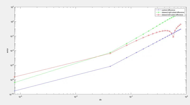
fig: plot for the comparison of dx and error of the each case.
In the above plot the blue line indicate the errors of the central differencing in the only the low percentage of the error will be plotted. but in case above two line are someward more percentages of errors compared to the central differencing skew.
MAIN CODE:
clear all
close all
clc
x=pi/3;
f=exp(x)*cos(x);
dx=linspace(pi/4,pi/4000,20);
analytical_derivative = -2*exp(x)*sin(x);
for i=1:length(dx)
    central_error(i) = fourth_order_central_differencing(analytical_derivative,x,dx(i));
    skewed_right_error(i) = fourth_order_right_sided_skew(analytical_derivative,x,dx(i));
    skewed_left_error(i) = fourth_order_left_sided_skew(analytical_derivative,x,dx(i));
end
%plotting
figure(1)
title('Differencing scheme comparison')
loglog(dx,central_error,'color','b','marker','+')
hold on
plot(dx,skewed_right_error,'color','g','marker','*')
hold on
plot(dx,skewed_left_error,'color','r','marker','>')
xlabel('dx')
ylabel('error')
legend('central difference','skewed right sided difference','skewed left sided difference')
FUNCTION CODE CENTRAL DIFFERENCING:
function error = fourth_order_central_differencing(analytical_derivative,x,dx)
%central differencing=a*f(x-2*dx)+b*f(x-dx)+c*f(x)+d*f(x+dx)+e*f(x+2*dx)
%analytical_derivative = -2*exp(x)*sin(x);
A = [1 1 1 1 1;-2 -1 0 1 2;4/2 1/2 0 1/2 4/2; -8/6 -1/6 0 1/6 8/6;16/24 1/24 0 1/24 16/24]
B = [0;0;1;0;0]
X = inv(A)*B
central_differencing=((X(1)*exp(x-2*dx)*cos(x-2*dx))+(X(2)*exp(x-dx)*cos(x-dx))+(X(3)*exp(x)*cos(x))+(X(4)*exp(x+dx)*cos(x+dx))+(X(5)*exp(x+2*dx)*cos(x+2*dx)))/(dx^2);
error=abs(analytical_derivative-central_differencing);
end
FUNCTION CODE RIGHT SIDED SKEW:
function error = fourth_order_right_sided_skew(analytical_derivative,x,dx)
%skewed right sided difference=(a*f(x)+b*f(x+dx)+c*f(x+2*dx)+d*f(x+3*dx)+e*f(x+4*dx)+g*f(x+5*dx))/(dx^2)
%analytical_derivative = -2*exp(x)*sin(x);
C = [1 1 1 1 1 1;0 1 2 3 4 5;0 1/2 2 9/2 16/2 25/2;0 1/6 8/6 27/6 64/6 125/6;0 1/24 16/24 81/24 256/24 625/24;0 1/120 32/120 243/120 1024/120 3125/120]
D = [0;0;1;0;0;0]
Y = inv(C)*D
skewed_right_differencing=((Y(1)*exp(x)*cos(x))+(Y(2)*exp(x+dx)*cos(x+dx))+(Y(3)*exp(x+2*dx)*cos(x+2*dx))+(Y(4)*exp(x+3*dx)*cos(x+3*dx))+(Y(5)*exp(x+4*dx)*cos(x+4*dx))+(Y(6)*exp(x+5*dx)*cos(x+5*dx)))/(dx^2);
error=abs(analytical_derivative-skewed_right_differencing);
end
FUNCTION CODE FOR LEFT SIDED SKEW:
function error = fourth_order_left_sided_skew(analytical_derivative,x,dx)
%skewed left sided difference=(a*f(x-5*dx)+b*f(x-4*dx)+c*f(x-3*dx)+d*f(x-2*dx)+e*f(x-dx)+g*f(x))/(dx^2)
%analytical_derivative = -2*exp(x)*sin(x);
E = [1 1 1 1 1 1;-5 -4 -3 -2 -1 0;25/2 16/2 9/2 4/2 1/2 0;-125/6 -64/6 -27/6 -8/6 -1/6 0;625/24 256/24 81/24 16/24 1/24 0;-3125/120 -1024/120 -243/120 -32/120 -1/120 0]
F = [0;0;1;0;0;0]
Z = inv(E)*F
skewed_left_differencing=((Z(1)*exp(x-5*dx)*cos(x-5*dx))+(Z(2)*exp(x-4*dx)*cos(x-4*dx))+(Z(3)*exp(x-3*dx)*cos(x-3*dx)+(Z(4)*exp(x-2*dx)*cos(x-2*dx))+(Z(5)*exp(x-dx)*cos(x-dx))+(Z(6)*exp(x)*cos(x))))/(dx^2);
error=abs(analytical_derivative-skewed_left_differencing);
end
CONCLUSION:
Her i conclude that the plot the blue line indicate the errors of the central differencing in the only the low percentage of the error will be plotted. but in case above two line are someward more percentages of errors compared to the central differencing skew. hence deriving 4th order approximation of a 2nd order derivative using Taylor Table method is done by using the MATLAB.
Describe why a skewed scheme is useful? What can a skewed scheme do that a CD scheme cannot?
1.Calculate error at boundary,we cannot apply central diiference sheme since it require value from both end.
2.Calculate error at the boundary we can apply skewed diference scheme only.
3.But we applyb the skewed at the boundary but we can get the accurate valves.
4.central differencing skewed scheme will the accurate valve and the very low error percentage.