Week 3.5 - Deriving 4th order approximation of a 2nd order derivative using Taylor Table method

AIM:

The goal is to approximate a second-order derivative at the fourth-order level by means of a central differencing scheme, a skewed right-sided difference, and a skewed left-sided difference, all generated by use of the Taylor table approach, and then to compare these approximations to the analytical derivative of the provided function.

SCHEME DERIVATIONS:

CENTRAL DIFFERENCING SCHEME:

NO OF NODES:

The number of nodes = p+q-1

Where, p is order of derivative.

q is order of approximations.

The no of nodes = 2+4-1 =>5.

DERIVATION:

In order to arrive at an approximation of the fourth order for the second order derivative, we will begin with these approximations.

taylor series derivation for the above terms,

Expanding each of the terms in equation (1) in a similar manner, the results are presented in the form of a table and are analysed using the Taylor table approach.

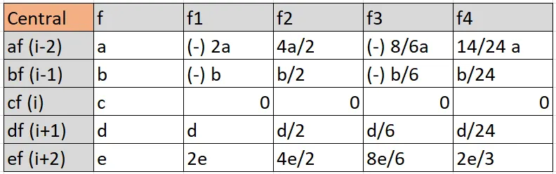
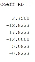
Using the matrix inversion method, we are able to solve the linear equation that we acquired from the table above.

A.X = B

X = inv(A)*B

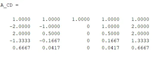
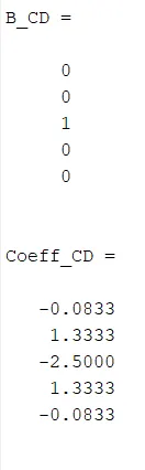
Similarly we have to follow the same steps for Skewed Righ and Left hand Differencing Scheme.

SKEWED RIGHT HAND DIFFERENCE SCHEME:

NO OF NODES:

The number of nodes = p+q

Where, p is order of derivative.

q is order of approximations.

The no of nodes = 2+4 =>6.

DERIVATION:

In order to arrive at an approximation of the fourth order for the second order derivative, we will begin with these approximations.

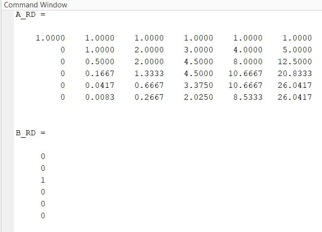
SKEWED LEFT HAND DIFFERENCE SCHEME:

NO OF NODES:

The number of nodes = p+q

Where, p is order of derivative.

q is order of approximations.

The no of nodes = 2+4 =>6.

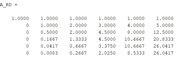
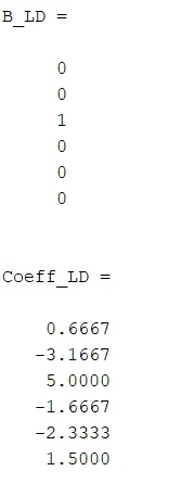
DERIVATION:

In order to arrive at an approximation of the fourth order for the second order derivative, we will begin with these approximations.

close all
clear all
clc

% value of x & dx
x= pi/3;
dx= linspace(pi/3,pi/3000,20);
% dx = pi/4;
analytical_derivate = -2*(exp(x))*sin(x);

A_CD = [1 1 1 1 1; -2 -1 0 1 2; 2 0.5 0 0.5 2; -4/3 -1/6 0 1/6 4/3; 2/3 1/24 0 1/24 2/3];
B_CD = [0; 0; 1; 0; 0];
Coeff_CD = linsolve(A_CD,B_CD);


A_RD = [1 1 1 1 1 1; 0 1 2 3 4 5; 0 0.5 2 9/2 16/2 25/2; 0 1/6 8/6 27/6 64/6 125/6; 0 1/24 16/24 81/24 256/24 625/24; 0 1/120 32/120 243/120 1024/120 3125/120];
B_RD = [0; 0; 1; 0; 0; 0];
Coeff_RD = linsolve(A_RD,B_RD);

A_LD = [1 1 1 1 1 1; -5 -4 -3 -2 -1 0; 25/2 16/2 9/2 4/2 1/2 0; -125/6 -64/6 -27/6 -8/6 -1/6 0; 652/24 256/24 81/24 16/24 1/24 0; -3125/120 -1024/120 -243/120 -32/120 -1/120 0];
B_LD = [0; 0; 1; 0; 0; 0];
Coeff_LD = linsolve(A_LD,B_LD);



f = @(x) exp(x)*cos(x);


% loop for calulating errors
for i= 1:length(dx)
   der_central_diff = (Coeff_CD(1,1)*f(x-2*dx(i)) + Coeff_CD(2,1)*f(x-1*dx(i)) + Coeff_CD(3,1)*f(x) + Coeff_CD(4,1)*f(x+1*dx(i)) + Coeff_CD(5,1)*f(x+2*dx(i)))/(dx(i)^2);
   error_CD (i) = abs(analytical_derivate - der_central_diff);
    
der_RS_diff = (Coeff_RD(1,1)*f(x) + Coeff_RD(2,1)*f(x+1*dx(i)) + Coeff_RD(3,1)*f(x+2*dx(i)) + Coeff_RD(4,1)*f(x+3*dx(i)) + Coeff_RD(5,1)*f(x+4*dx(i)) + Coeff_RD(6,1)*f(x+5*dx(i)))/(dx(i)^2);
error_RD (i) = abs(analytical_derivate - der_RS_diff);

der_LS_diff = (Coeff_LD(1,1)*f(x-5*dx(i)) + Coeff_LD(2,1)*f(x-4*dx(i)) + Coeff_LD(3,1)*f(x-3*dx(i)) + Coeff_LD(4,1)*f(x-2*dx(i)) + Coeff_LD(5,1)*f(x-1*dx(i)) + Coeff_LD(6,1)*f((x)))/(dx(i)^2);
error_LD (i) = abs(analytical_derivate - der_LS_diff);
end
figure(1);
loglog(dx,error_CD, 'r', 'linewidth',2);
hold on;
loglog(dx,error_RD, 'g', 'linewidth',2);
hold on;
loglog(dx,error_LD, 'b', 'linewidth',2);
xlabel('range of dx')
ylabel('truncation error')
title('range of dx vs error')
legend('central differencing','skewed right sided difference','skewed left sided difference','location','northwest');


figure(2);
plot(dx,error_CD, 'r', 'linewidth',2);
hold on;
plot(dx,error_RD, 'b', 'linewidth',2);
hold on;
plot(dx,error_LD,'m', 'linewidth',2);

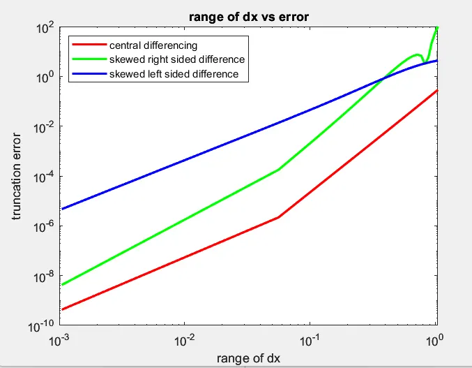
OUTPUT:

• 

EXPLANATION:

• Initially, the equations for each of the schemes were worked out on paper; subsequently, in order to acquire the coefficients of the equations, those equations were worked out using MATLAB (you can see in code).
  
• The user will be prompted to enter the value for x as well as the range for dx, and both of these values will be used in the same code by using the for loop instead of making functions.
  
• The primary code will provide a comprehensive analysis of the various error rates produced by each method.
• The purpose of utilising central, right hand skewed, and left hand skewed schemes is to get a better level of approximation at the nodes that do not have a left or right point (they are starting point).
  
• Using the right hand scheme and the left hand technique together will allow one to obtain the higher order approximation.

CONCLUSION

• The plot demonstrates that the central scheme is superior to the two skewed systems in terms of both efficiency and accuracy. This is because the central scheme uses information from both sides to arrive both an approximation and an accurate conclusion.
• On the other hand, skewed schemes are successful in locations where there is insufficient information on both sides. For instance, in a situation in which we do not know either the previous or the forward points, we can use left handed or right handed skewed schemes, depending on which is more appropriate, to solve the problem.