Week 3.5 - Deriving 4th order approximation of a 2nd order derivative using Taylor Table method

CHALLENGE - 3.5 : Deriving 4th Order Approximation of a 2nd Order Derivative Using Taylor Table Method

AIM:

To derive fourth order approximation of a 2nd order derivative using Taylor Table method for Central difference method, Skewed right-sided difference method and Skewed left-sided difference method

OBJECTIVES:

1. To derive fourth order approximation of a 2nd order derivative for Central difference method, Skewed right-sided difference method and Skewed left-sided difference method.
2. To write a Matlab program to evaluate the second-order derivative of the analytical function exp(x)*cos(x) and compare it with the 3 numerical approximations that derived.
3. To plot a comparison plot between the absolute error between the above-mentioned schemes.

THEORY:

1. Central Difference Method

In Central difference method the derivative of a fuction is defined from the values of fuction on both side of point at which the derivative of the fuction is to be evaluated.

For central difference method the order of accuracy can be evaluated by using the below equation.

The order of accuracy P = Number of nodes in the stencil N - order of derivative Q + 1 for central schemes

So, in this case P = 4, Q = 2.

=> Number of nodes in the stencil N = P + Q - 1

N = 4+2-1 = 5 Points.

General form of the expression with 5 nodes for Central difference method is

`(del^2phi)/(delx^2)= af(i-2)+bf(i-1)+cf(i)+df(i+1)+ef(i+2)`

	f(i)	∆x f'(i)	∆x^2 f''(i)	∆x^3 f'''(i)	∆x^4 f''''(i)
af(i-2)	a	a*-2	a*(4/2!)	a*-(8/3!)	a*16/4!
bf(i-1)	b	b*-1	b/(2!)	b/-(3!)	b/4!
cf(i)	c	0	0	0	0
df(i+1)	d	d	d/(2!)	d/(3!)	d/4!
ef(i+2)	e	e*2	e*(4/2!)	e*(8/3!)	e*16/4!
Sum of Coeff	0	0	1	0	0

Rewriting the above table into matrix form

`[[1,1,1,1,1], [-2,-1,0,1,2],[2, 1/2, 0, 1/2, 2], [-4/3,-1/6,0,1/6,4/3], [2/3,1/24,0,1/24,2/3]]*[[a],[b],[c],[d],[e]]=[[0],[0],[1],[0],[0]]`

Solving the above equation we get:

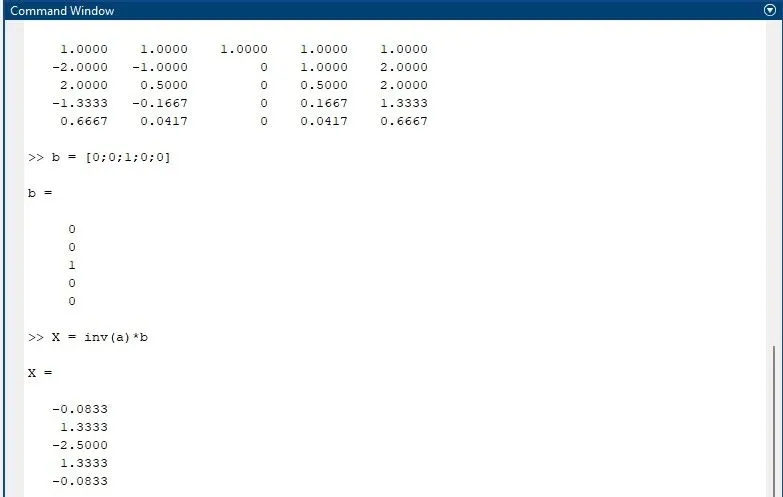
a = -0.8333, b = 1.333, c = -2.5, d = 1.333, e = -0.0833

`(del^2phi)/(delx^2)= -0.8333f(i-2)+1.333f(i-1)-2.5f(i)+1.3333f(i+1)-0.8333f(i+2)`

2. Skewed right-sided difference Method

In Central difference method the derivative of a fuction is defined from the values of fuction on right side/forward of the point at which the derivative of the fuction is to be evaluated.

For right-sided difference method the order of accuracy can be evaluated by using the below equation.

The order of accuracy P = Number of nodes in the stencil N - order of derivative Q

So, in this case P = 4, Q = 2.

=> Number of nodes in the stencil N = P + Q

N = 4+2 = 6 Points.

General form of the expression with 6 nodes for Central difference method is

`(del^2phi)/(delx^2)= af(i)+bf(i+1)+cf(i+2)+df(i+3)+ef(i+4)+kf(i+5)`

	f(i)	∆x f'(i)	∆x^2 f''(i)	∆x^3 f'''(i)	∆x^4 f''''(i)	∆x^5 f'''''(i)
af(i)	a	0	0	0	0	0
bf(i+1)	b	b	b/(2!)	b/3!	b/4!	b/5!
cf(i+2)	c	2c	4c/2!	8c/3!	16c/4!	32c/5!
df(i+3)	d	3d	9d/(2!)	27d/(3!)	81d/4!	243d/5!
ef(i+4)	e	4e	16e/2!	64e/3!	256e/4!	1024e/5!
kf(i+5)	k	5k	25k/2!	125k/3!	625k/4!	3125k/5!
Sum of Coeff	0	0	1	0	0	0

Rewriting the above table into matrix form

`[[1,1,1,1,1,1], [0,1,2,3,4,5],[0,1/2, 2, 9/2, 8,25/2], [0,1/6,8/6,27/6,64/6,125/6], [0,1/24,16/24,81/24,256/24,625/24],[0,1/120,32/120,243/120,1024/120,3125/120]]*[[a],[b],[c],[d],[e],[k]]=[[0],[0],[1],[0],[0],[0]]`

Solving the above equation we get:

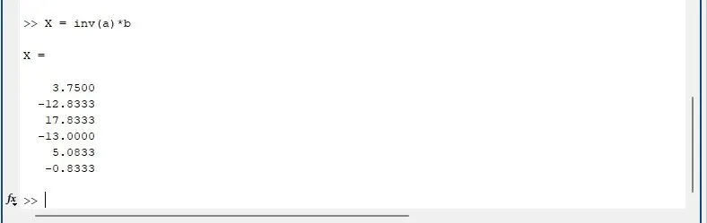
a = 3.75, b = -12.8333, c = 17.8333, d = -13, e = 5.0833, k = -0.8333

`(del^2phi)/(delx^2)= 3.75f(i)-12.8333f(i+1)+17.8333f(i+2)-13f(i+3)+5.0833f(i+4)-0.8333f(i+5)`

3. Skewed left-sided difference Method

In Central difference method the derivative of a fuction is defined from the values of fuction on left side/backward of the point at which the derivative of the fuction is to be evaluated.

For right-sided difference method the order of accuracy can be evaluated by using the below equation.

The order of accuracy P = Number of nodes in the stencil N - order of derivative Q

So, in this case P = 4, Q = 2.

=> Number of nodes in the stencil N = P + Q

N = 4+2 = 6 Points.

General form of the expression with 6 nodes for Central difference method is

`(del^2phi)/(delx^2)= af(i-5)+bf(i-4)+cf(i-3)+df(i-2)+ef(i-1)+kf(i)`

	f(i)	∆x f'(i)	∆x^2 f''(i)	∆x^3 f'''(i)	∆x^4 f''''(i)	∆x^5 f'''''(i)
af(i-5)	a	-5a	25a/2!	-125a/3!	625a/4!	-3125a/5!0
bf(i-4)	b	-4b	16b/2!	-64b/3!	256b/4!	-1024b/5!
cf(i-3)	c	-3c	9c/2!	-27c/3!	81c/4!	-243c/5!
df(i-2)	d	-2d	4d/(2!)	-8d/(3!)	16d/4!	-32d/5!
ef(i-1)	e	-e	e/2!	-e/3!	e/4!	-e/5!
kf(i)	k	0	0	0	0	0
Sum of Coeff	0	0	1	0	0	0

Rewriting the above table into matrix form

`[[1,1,1,1,1,1], [-5,-4,-3,-2,-1,0],[25/2,8,9/2,2,1/2,0], [-125/6,-64/6,-27/6,-8/6,-1/6,0], [625/24,256/24,81/24,16/24,1/24,0],[-3125/120,-1024/120,-243/120,-32/120,-1/120,0]]*[[a],[b],[c],[d],[e],[k]]=[[0],[0],[1],[0],[0],[0]]`

Solving the above equation we get:

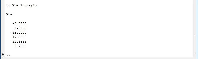
a = -0.8333, b = 5.0833, c = -13, d = 17.8333 , e = -12.8333, k = 3.75

`(del^2phi)/(delx^2)= -0.8333f(i-5)+5.08333f(i-4)-13f(i-3)+17.8333f(i-2)-12.8333f(i-1)+3.75f(i)`

Solve the expression exp(x)*cos(x) using the above 3 equations by using Matlab program.

PROCEDURE:

Procedure for matlab program is mentioned below.

1. Program is started by using the general commands clear all, close all and clc to clear and close all the pre-occupied operations of Matlab.
2. Provide the input codition that value of x = pi/2 and dx by using linspace command
   dx = linspace(pi/40,pi/4000,30)
3. Call the fuctions of Central_Diff, Forward_Diff and Backward_Diff.
4. Define the functions Central_Diff, Forward_Diff and Backward_Diff in a new file and save the files with same function name in same folder where the main program is saved.
5. Evaluate the expression analytically and by using above mentioned equations then find the absolute error.
6. Plot this camparison of anlytical solution and numerical solution by using plot command for all the three cases.
7. Provide labels and legends to the plot.
8. Save and Run the file.

The main program which is created on Matlab is attached below.

% Program to solve 2nd order derivative with Central diff, Forward and
% backward with 4th order approx

clear all 
close all
clc

% Input value of X and dx
x = pi/2;
dx = linspace(pi/40,pi/4000,30);


% For loop to calculate error for different value of dx
for i = 1:30

 error_CD(i) = Central_Diff(x, dx(i));
 error_FD(i) = Forward_Diff(x, dx(i));
 error_BD(i) = Backward_Diff(x, dx(i));

end

% Plotting

figure(1)
loglog(dx,error_CD,"Color",'r')
hold on
loglog(dx,error_FD,"Color",'b')
hold on
loglog(dx,error_BD,"Color",'g')
xlabel('dx');
ylabel('Absolute-Error');
legend('Central Differencing', 'Skewed right-sided difference', 'Skewed left-sided difference')

• Function for Central Difference Method

% Function of Central Differencing

function error_C_D = Central_Diff(x, dx)

analytical = -2*exp(x)*sin(x);

a = [1 1 1 1 1; -2 -1 0 1 2; 2 1/2 0 1/2 2; -4/3 -1/6 0 1/6 4/3; 2/3 1/24 0 1/24 2/3]
b = [0; 0; 1; 0; 0];
X = inv(a)*b;

numerical_c_d = (((X(1))*(exp(x-(2*dx)))*(cos(x-(2*dx))))+((X(2))*(exp(x-dx))*(cos(x-dx)))+((X(3))*(exp(x))*(cos(x)))+((X(4))*(exp(x+dx))*(cos(x+dx)))+((X(5))*(exp(x+(2*dx)))*(cos(x+(2*dx)))))/(dx^2);

error_C_D = abs(analytical-numerical_c_d);

end

• Function for Skewed right-sided Difference Method

% Function of Forward Differencing

function error_F_D = Forward_Diff(x, dx)

analytical = -2*exp(x)*sin(x);

a = [1 1 1 1 1 1; 0 1 2 3 4 5; 0 1/2 2 9/2 8 25/2; 0 1/6 8/6 27/6 64/6 125/6; 0 1/24 16/24 81/24 256/24 625/24; 0 1/120 32/120 243/120 1024/120 3125/120];
b = [0; 0; 1; 0; 0; 0];
X = inv(a)*b;


numerical_f_d = (((X(1))*((exp(x))*(cos(x))))+((X(2))*((exp(x+dx))*(cos(x+dx))))+((X(3))*((exp(x+(2*dx)))*(cos(x+(2*dx)))))+((X(4))*((exp(x+(3*dx)))*(cos(x+(3*dx)))))+((X(5))*((exp(x+(4*dx)))*(cos(x+(4*dx)))))+((X(6))*((exp(x+(5*dx)))*(cos(x+(5*dx))))))/(dx^2);
error_F_D = abs(analytical-numerical_f_d);

end

• Function for Skewed left-sided Difference Method

% Function of Backward Differencing

function error_B_D = Backward_Diff(x, dx)

analytical = -2*exp(x)*sin(x);

a = [1 1 1 1 1 1; -5 -4 -3 -2 -1 0; 25/2 8 9/2 2 1/2 0; -125/6 -64/6 -27/6 -8/6 -1/6 0; 625/24 256/24 81/24 16/24 1/24 0; -3125/120 -1024/120 -243/120 -32/120 -1/120 0];
b = [0; 0; 1; 0; 0; 0];
X = inv(a)*b;

numerical_b_d = (((X(1))*((exp(x-(5*dx)))*(cos(x-(5*dx)))))+((X(2))*((exp(x-(4*dx)))*(cos(x-(4*dx)))))+((X(3))*((exp(x-(3*dx)))*(cos(x-(3*dx)))))+((X(4))*((exp(x-(2*dx)))*(cos(x-(2*dx)))))+((X(5))*((exp(x-dx))*(cos(x-dx))))+((X(6))*((exp(x))*(cos(x)))))/(dx^2);

error_B_D = abs(analytical-numerical_b_d);

end

Results obtained are discussed in the below session.

RESULTS AND DISCUSSION:

The comparison plot obtained after executing the above code is shown below:

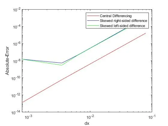
From the above plot it is evident that central difference method provide much accurate results as compared to skewed left sided and skewed right sided cases.

It is also evident that when step size is decreased below a particular value error starts increasing. It is mainly because of the presents of round off error. That is with decrease in step size trucation error decreases but round off error increases. So for the evalution always use the optimum value of step size which results in minimum error.

• why a skewed scheme is useful? What can a skewed scheme do that a CD scheme cannot?

Even though Central difference method provide accurate method as compared to other method. Skewed scheme is useful when there is unavailability of datas on either one side of the points to be evaluated. In such case central difference method cannot be employed.

For evaluating a point on the bounday central difference scheme cannot be employed in such scenario skewed schemes are recommended.

CONCLUSION:

Fourth order approximation of a 2nd order derivative using Taylor Table method for Central difference method, Skewed right-sided difference method and Skewed left-sided difference method have been derived and a matlab program to evaluate an expression using these methods are also carried out. A comparison plot of absolute errors obtained for all the three schemes are discussed.