Week 3.5 - Deriving 4th order approximation of a 2nd order derivative using Taylor Table method

AIM:- Write a MATLAB Program to evaluate the second-order derivative of the analytical function

OBJECTIVE:

- To write a program and evaluate the second-order derivative of the analytical function exp(x)*cos(x)

- Understand central differencing scheme, skewed right difference scheme, and skewed left difference scheme with the help of Taylor table

- Compare the results for 3 numerical approximations.

Procedure:-

The function given to solve for;

`f(x)=exp(x)⋅cos(x)`

Analytical derivative -

`f'(x)=exp(x)⋅cos(x)−exp(x)⋅sin(x)`

`f''(x)=−2⋅exp(x)⋅sin(x)`

Numerical Solution -
Now we are doing the 4rth order approximation for the second-order derivative of the above function, considering for range of step size dx = `[pi/40, pi/4000,200].` and `x=pi/3`

The schemes used for the approximation are-

• Forward Skewed Differencing
• Backward Skewed Differencing
• Central Differencing

The number of grid points required for the accuracy of the differencing can be calculated as,

Forward and Backward Skewed,
N = P + Q = 4 + 2 = 6

and for central differencing,
N = P + Q - 1 = 4 + 2 - 1 = 5

Where,
P = Order of accuracy
N = Number of nodes in the stencil
Q = Order of derivative

# Now Deriving the Equations for the 4rth Order Approximation of 2nd Order Derivative using Taylor Table Method -

1. Forward Skewed Differencing

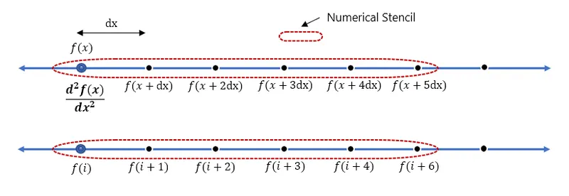
Here, the number of grid points are, N=6
The equation can be written as,

`f''(x) = a.f(i)+b.f(i+1)+c.f(i+2)+d.f(i+3)+e.f(i+4)+g.f(i+5)`

Using the Taylor Series of approximation Method,

	`f(x)`	`f'(x) .dx/(1!)`	`f''(x) .(dx)^2/(2!)`	`f'''(x) .(dx)^3/(3!)`	`f''''(x) .(dx)^4/(4!)/(4!)`	`f'''''(x) .(dx)^5/(5!)`
`a.f_(i)`	a	0	0	0	0	0
`b.f_(i+1)`	b	b	b	b	b	b
`c.f_(i+2)`	c	2c	4c	8c	16c	32c
`d.f_(i+3)`	d	3d	9d	27d	81d	243d
`e.f_(i+4)`	e	4e	16e	64e	256e	1024e
`g.f_(i+5)`	g	5g	25g	125g	625g	3125g
`sum = (d^2f(x))/dx^2`	0	0	1	0	0	0

As we know, `delx^4` denotes the truncation error, and the order of the truncation error {`0(delx^4)`} is '4'.
Since we know that the order of approximation is defined by the truncation error term. Therefore, we can say that our skewed right-sided difference scheme is of 4th order accurate.

In Matrix Form-

`[[1,1,1,1,1,1],[0,1,2,3,4,5],[0,1,4,9,16,25],[0,1,8,27,64,125],[0,1,16,81,256,625],[0,1,32,243,1024,3125]] *` `[[a],[b],[c],[d],[e],[g]]` = `[[0],[0],[1],[0],[0],[0]]`

On solving for the unknowns,

`[[a],[b],[c],[d],[e],[g]] = [[3.7500],[-12.833],[17.833],[-13],[5.0833],[-0.833]]`

Therefore the Equation for the 4rth order appx. of 2nd order derivative with Forward skewed Differencing

`f''(x)=(3.7500).f(i)+(−12.833).f(i+1)+(17.833).f(i+2)+(-13).f(i+3)+(5.0833).f(i+4)+(−0.833).f(i+5)`

2. Backward Skewed Differencing

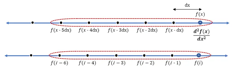
Here, the number of grid points are, N=6

The equation will be,

`f''(x) = a.f(i)+b.f(i-1)+c.f(i-2)+d.f(i-3)+e.f(i-4)+g.f(i-5)`

Using the Taylor Series of approximation Method,

	`f(x)`	`f'(x) .dx/(1!)`	`f''(x) .(dx)^2/(2!)`	`f'''(x) .(dx)^3/(3!)`	`f''''(x) .(dx)^4/(4!)/(4!)`	`f'''''(x) .(dx)^5/(5!)`
`a.f_(i)`	a	0	0	0	0	0
`b.f_(i-1)`	b	-b	b	-b	b	-b
`c.f_(i-2)`	c	-2c	4c	-8c	16c	-32c
`d.f_(i-3)`	d	-3d	9d	-27d	81d	-243d
`e.f_(i-4)`	e	-4e	16e	-64e	256e	-1024e
`g.f_(i-5)`	g	-5g	25g	-125g	625g	-3125g
`sum = (d^2f(x))/dx^2`	0	0	1	0	0	0

- The order of the truncation error {`0(delx^4)`} is '4'.
- Since we know that the order of approximation is defined by the truncation error term. Therefore, we can say that our skewed right-sided difference scheme is of 4th order accurate.

In Matrix Form-

`[[1,1,1,1,1,1],[0,-1,-2,-3,-4,-5],[0,1,4,9,16,25],[0,-1,-8,-27,-64,-125],[0,1,16,81,256,625],[0,-1,-32,-243,-1024,-3125]] *` `[[a],[b],[c],[d],[e],[g]]` = `[[0],[0],[1],[0],[0],[0]]`

On solving for the unknowns,

`[[a],[b],[c],[d],[e],[g]] = [[3.7500],[-12.833],[17.833],[-13],[5.0833],[-0.833]]`

Therefore the Equation for the 4rth order appx. of 2nd order derivative with Backward skewed Differencing,

`f''(x)=(3.7500).f(i)+(−12.833).f(i−1)+(17.833).f(i−2)+(−13).f(i−3)+(5.0833).f(i−4)+(−0.833).f(i−5)`

3. Central Differencing

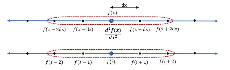
Here, the number of grid points are, N=5

`f''(x) = a.f(i−2)+b.f(i−1)+c.f(i)+d.f(i+1)+e.f(i+2)`

Using the Taylor Series of approximation Method,

	`f(x)`	`f'(x) .dx/(1!)`	`f''(x) .(dx)^2/(2!)`	`f'''(x) .(dx)^3/(3!)`	`f''''(x) .(dx)^4/(4!)/(4!)`	`f'''''(x) .(dx)^5/(5!)`
`a.f_(i-2)`	a	-2a	4a	-8a	16	32
`b.f_(i-1)`	b	-b	b	-b	b	-b
`c.f_(i)`	c	0	0	0	0	0
`a.f_(i+1)`	d	d	d	d	d	d
`a.f_(i+2)`	e	2e	4e	8e	16e	32e
`sum = (d^2f(x))/dx^2`	0	0	1	0	0	--

In Matrix Form-

`[[1,1,1,1,1],[-2,-1,0,1,2],[4,1,0,1,4],[-8,-1,0,1,8],[16,1,0,1,16]]` * `[[a],[b],[c],[d],[e]]` = `[[0],[0],[1],[0],[0]]`

On solving,

`[[a],[b],[c],[d],[e]]` = `[[-0.0833],[1.3333],[-2.50],[1.3333],[-0.0833]]`

Therefore the Equation for the 4rth order appx. of 2nd order derivative with Central Differencing,

`f''(x)=(−0.0833).f(i−2)+(1.333).f(i−1)+(−2.5).f(i)+(1.333).f(i+1)+(−0.0833).f(i+2)`

MATLAB Program:-

clear all
close all
clc



% Right skewed scheme
A = [1 1 1 1 1 1; 0 1 2 3 4 5; 0 1/2 2 9/2 8 25/2; 0 1/6 4/3 9/2 32/3 125/6; 0 1/24 2/3 27/8 32/3 625/24; 0 1/120 4/15 81/40 128/15 625/24] ;

B = [0; 0; 1; 0; 0; 0];

R = inv(A)*B;

% Left skewed scheme
M = [1 1 1 1 1 1; 0 -1 -2 -3 -4 -5; 0 1/2 2 9/2 8 25/2; 0 -1/6 -4/3 -9/2 -32/3 -125/6; 0 1/24 2/3 27/8 32/3 625/24; 0 -1/120 -4/15 -81/40 -128/15 -625/24] ;

N = [0; 0; 1; 0; 0; 0];

L = inv(M)*N;

% Central scheme
P = [1 1 1 1 1 ; -2 -1 0 1 2; 2 1/2 0 1/2 2; -4/3 -1/6 0 1/6 4/3; 2/3 1/24 0 1/24 2/3] ;

Q = [0; 0; 1; 0; 0];

Z = inv(P)*Q;


x = pi/3;

dx = linspace(pi/400,pi/400000,20);

% function f(x) = e^x*cos(x)
% analytical first derivative =  e^xcos(x) - e^x*sin(x) || Chain rule :
% f'(uv) = u'v + uv'

% analytical second derivative = -2*e^x*cos(x)

analytical_derivative = -2*exp(x)*sin(x);

% Function handle 
f = @(x) exp(x).*cos(x);


right_skewed_scheme =  (R(1)*f(x) + R(2)*f(x+dx) + R(3)*f(x+(2*dx)) + R(4)*f(x+(3*dx)) + R(5)*f(x+(4*dx)) + R(6)*f(x+(5*dx)))./(dx.^2);

left_skewed_scheme =  (R(1)*f(x) + R(2)*f(x-dx) + R(3)*f(x-(2*dx)) + R(4)*f(x-(3*dx)) + R(5)*f(x-(4*dx)) + R(6)*f(x-(5*dx)))./(dx.^2);

central_scheme = (Z(1)*f(x-(2*dx)) + Z(2)*f(x-dx) + Z(3)*f(x) + Z(4)*f(x+dx) + Z(5)*f(x+(2*dx)))./(dx.^2);

% Error in Scheme
error_right_skewed_scheme = abs(right_skewed_scheme-analytical_derivative);
error_left_skewed_scheme = abs(left_skewed_scheme-analytical_derivative);
error_central_scheme = abs(central_scheme-analytical_derivative);

% Plotting
figure(1)
loglog(dx,error_right_skewed_scheme,'b',dx,error_left_skewed_scheme,'g',dx,error_central_scheme,'r');
legend('Error Right Skewed','Error Left Skewed','Error Central Scheme')
xlabel('dx')
ylabel('Error')
grid on

Result:-

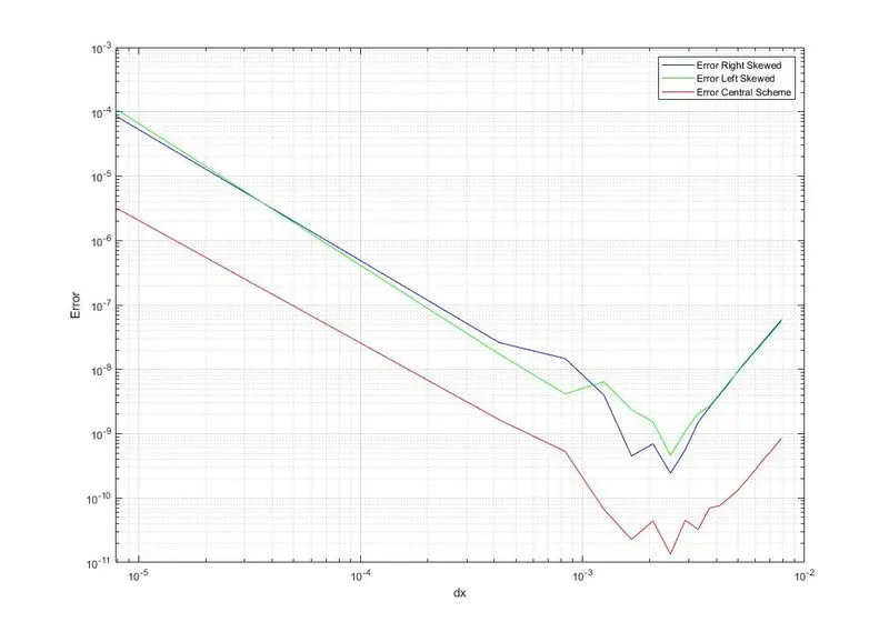
- Plotting is made between dx on the x-axis and errors on the y-axis.

- From the graph, shows that for the 4rth order approximation, the central differencing is more accurate i.e. having less error than the backward skewed and forward skewed differencing.

- Skewed right and left difference methods almost give the same results.

Conclusion:-

Central Differencing convergence rate is faster than all other differencing schemes.

Central Differencing is mostly used in the middle region of the grid space. Since it is symmetric and requires the same no. of nodes from both directions.

Ques- Why a skewed scheme is useful? What can a skewed scheme do that a CD scheme cannot do?

skewed differencing schemes require the information available at the next neighboring points on one side from the point of consideration either left or right to give the approximation value.

And therefore, for the region closer to the boundaries the forward & backward skewed Differencing is used.