Deriving 4th order approximation of a 2nd order derivative using Taylor Table method

Aim:

To calculate the 2nd order derivative with 4th order approximation with Central Difference and Skewed Difference Schemes using MATLAB

Given function:

`f(x)=exp(x)**cos(x)`

Formula:

Exact solution:

`f''(x)=-2 sin(x)**exp(x)`

Number of nodes (CDS):

`n=p+q-1`

Number of nodes(Skewed Schemes):

`n=p+q`

where

p - Order of derivative

q - Order of approximation

Central Difference Scheme (4th order approximation)

`f''(x)=(af(x)_(i-2)+bf(x)_(i-1)+cf(x)_(i)+df(x)_(i+1)+ef(x)_(i+2))/(Deltax)^2+O((Deltax)^4)`

Skewed Right-Sided Scheme

`f''(x)=(af(x)_(i)+bf(x)_(i+1)+cf(x)_(i+2)+df(x)_(i+3)+ef(x)_(i+4)+gf(x)_(i+5))/(Deltax)^2+O((Deltax)^4)`

Skewed Left-Sided Scheme

`f''(x)=(af(x)_(i)+bf(x)_(i-1)+cf(x)_(i-2)+df(x)_(i-3)+ef(x)_(i-4)+gf(x)_(i-5))/(Deltax)^2+O((Deltax)^4)`

Matlab code:

clear all
close all
clc

x = pi/4;
dx = linspace(pi/20,pi/4000,40);

% Exact derivative using differentiation
exact = -2*exp(x)*sin(x);

% Coefficients of all terms in Taylor series for Central Difference Scheme 
for i = 0:4
    for j = -2:2
        A1(i+1,j+3) = (j^i)/(factorial(i));
    end
end

% Coefficients of all terms in Taylor series for Skewed Right Sided and Skewed Left Sided Scheme 
for i = 0:5
    for j = 0:5
        A2(i+1,j+1) = (j^i)/factorial(i);
        A3(i+1,j+1) = ((-j)^i)/factorial(i);
    end    
end

syms a b c d e g
% Central Differencing Scheme multiplying matrix elements with coefficient variables
eqn1 = A1*[a;b;c;d;e];
% Skewed Right Sided Scheme multiplying matrix elements with coefficient variables
eqn2 = A2*[a;b;c;d;e;g];
% Skewed Left Sided Scheme multiplying matrix elements with coefficient variables
eqn3 = A3*[a;b;c;d;e;g];

vars = [a b c d e];
vars2 = [a b c d e g];

% CDS equations
eqns1 = [eqn1(1)==0,eqn1(2)==0,eqn1(3)==1,eqn1(4)==0,eqn1(5)==0];
[C,D] = equationsToMatrix(eqns1, vars);

% Skewed Left Sided equations
eqns2 = [eqn2(1)==0,eqn2(2)==0,eqn2(3)==1,eqn2(4)==0,eqn2(5)==0,eqn2(6)==0];
[E,F] = equationsToMatrix(eqns2, vars2);

% Skewed Right Sided equations
eqns3 = [eqn3(1)==0,eqn3(2)==0,eqn3(3)==1,eqn3(4)==0,eqn3(5)==0,eqn3(6)==0];
[G,H] = equationsToMatrix(eqns3, vars2);

% Solving the equations
X1 = linsolve(C,D);
X2 = linsolve(E,F);
X3 = linsolve(G,H);

% Assigning 0 value
CDS = zeros(length(dx),1);
SR = zeros(length(dx),1);
SL = zeros(length(dx),1);


for j = 1:length(dx)
    
    for i = -2:2
        CDS(j) = CDS(j) + (X1(i+3)*exp(x+i*dx(j))*cos(x+i*dx(j)));
    end
    CDS(j) = CDS(j)/(dx(j)^2);
    % CDS error calculation
    error_cds(j) = abs(exact-CDS(j));
    
    for i = 0:5
        SR(j) = SR(j) + (X2(i+1)*exp(x+i*dx(j))*cos(x+i*dx(j)));
        SL(j) = SL(j) + (X3(i+1)*exp(x-i*dx(j))*cos(x-i*dx(j)));
        
    end
    SR(j) = SR(j)/(dx(j)^2);
    % Skewed right sided scheme error 
    error_sr(j) = abs(exact-SR(j));
    
    SL(j) = SL(j)/(dx(j)^2);
    % Skewed left sided scheme error
    error_sl(j) = abs(exact-SL(j));
    
end

% Plotting the log graph
figure(1);
loglog(dx,error_cds,'--mo')
hold on;
loglog(dx,error_sr,':bs','MarkerSize',10)
loglog(dx,error_sl,'-.r*')
legend('Central Difference Scheme','Skewed right sided difference','Skewed left sided difference','location','best')
title('Error comparison')
xlabel('dx')
ylabel('Error')

% Plotting the graph
figure(2);
plot(dx,error_cds,'--mo')
hold on;
plot(dx,error_sr,':bs','MarkerSize',10)
plot(dx,error_sl,'-.r*')
legend('Central Difference Scheme','Skewed right sided difference','Skewed left sided difference','location','best')
title('Error comparison')
xlabel('dx')
ylabel('Error')

Explanation:

• The values for x and dx are assigned
• The exact solution of the given fuction is found using direct differentiation
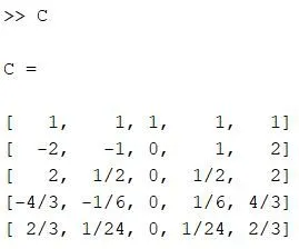
• Coefficients of all terms in Taylor series for Central Difference Scheme is found using nested for loops and stored in a 5x5 array (5 sets of equations since p+q-1 => 2+4-1=5 nodes)
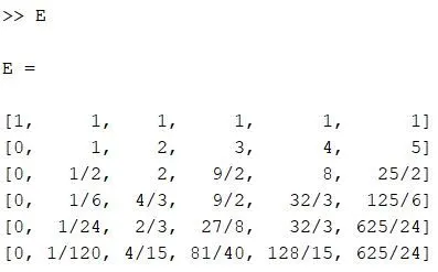
• Coefficients of all terms in Taylor series for Skewed Schemes are found using the same logic with variation in end values, and stored in a 6x6 array (6 sets of equations since p+q => 2+4=6 nodes)
• The matrices are multiplied to the unknown coefficients
• The expressions are equated to the values in such a way that the last term remaining is the second order derivative. The equations are then stored in one single variable namely eqns1, eqns2, eqns3 for CDS and Skewed schemes respectively
• Inbuilt function, equationsToMatrix(eqn,var) is used to convert the eqations into matrix forms
• Equations in the matrix form are solved using the inbuilt function linsolve() which takes in the tylors table matrix and the RHS (sum of the terms in taylor series so that all terms other than 2nd order derivative becomes 0) as input. The values of unknown coefficients are stored in arrays X1, X2, X3
• Initially the values of CDS, SR (Skewed Right-sided), SL (Skewed Left-sided) are assigned to 0, therefore no error occurs during the addition process. These variables are used to store the values of 2nd order derivative terms in an array for respective values of dx
• Value of given function is found for specified value of dx which is multiplied with the respective coefficients. Values for previous and next node terms are also found in the same manner and are added using a for loop. The outer for loop is executed over the length of dx, so that 2nd order derivatives for every values of dx is found.
• Error in the approximation is found by taking the absolute difference of found solution with the exact solution.
• Error plots for all the three schemes are plotted

After solving the equations for the unknown coefficient variables, the final equations were found to be

Central Difference Scheme (4th order approximation)

`f''(x)=(-f(x)_(i-2)+16f(x)_(i-1)-30f(x)_(i)+16f(x)_(i+1)-f(x)_(i+2))/(12(Deltax)^2)+O((Deltax)^4)`

Skewed Right-Sided Scheme

`f''(x)=(45f(x)_(i)-154f(x)_(i+1)+214f(x)_(i+2)-156f(x)_(i+3)+61f(x)_(i+4)-10f(x)_(i+5))/(12(Deltax)^2)+O((Deltax)^4)`

Skewed Left-Sided Scheme

`f''(x)=(45f(x)_(i)-154f(x)_(i-1)+214f(x)_(i-2)-156f(x)_(i-3)+61f(x)_(i-4)-10f(x)_(i-5))/(12(Deltax)^2)+O((Deltax)^4)`

Output:

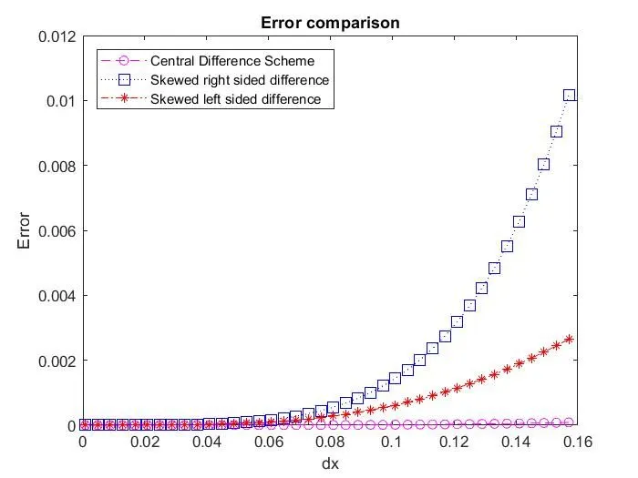
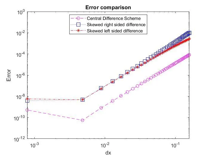
Log plot:

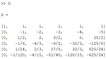
Taylors table matrices for CDS (C), Skewed Right-sided (E) and Skewed Left-sided (G) Schemes

Results:

• Central Difference Scheme for 2nd order derivative with 4th order approximation has the highest accuracy when compared to Skewed Left-sided and Skewed Right-sided Schemes.
• Skewed Left sided scheme yielding a better result than Skewed Right sided Scheme which is clearly visible in the log plot.
• For values of dx less than `10^-2` , the plot tends to deviate from the previous line. This is encountered because when the value of dx becomes so low, round off error comes into picture, which gives rise to the observed anomaly