Simple Pendulum Animation by Solving 2nd Order ODE

Aim:

Write a code to solve the 2nd order ODE govering the motion of a simple pendulum in MATLAB

Matlab Code:

Function (ode_func):

function [dtheta_dt]=ode_func(theta,b,g,l,m)
    %unknown variables
    theta1=theta(1);
    theta2=theta(2);

    %angular position
    dtheta1_dt=theta2;
    %angular velocity
    dtheta2_dt=-(b/m)*theta2-(g/l)*sin(theta1);
    %variable that stores the combined results of angular position and velocity
    dtheta_dt=[dtheta1_dt;dtheta2_dt];
end

Explanation:

1) This function is used to calculate the expression for the second order differential equation with the available constant values, and to store the first order and second order derivatives in a single array.

2) dtheta_dt array consists of 2 unknown variables (angular position and velocity), but has the required formulas to calculate them at a given time step.

3) The arguments of this fuction are theta (variable whose derivative is to be found), damping coefficient (b), acceleration due to gravity (g), length of the string (l) and mass of the bob (m).

Formula:

`(d^2theta)/dt^2+(b/m)(d theta)/dt + (g/l)sintheta=0`

θ₁=θ

θ₂=dθ₁/dt

where,

g = gravity in `m`/`s^2`

l = length of the pendulum in `m`

m = mass of the ball in `kg`

b = damping coefficient

Main Program (ode_main):

%ODE main
clear all
close all
clc

%constants
b=0.05; %damping coefficient
g=9.81; %acceleration due to gravity (m/s^2)
l=1; %length of string (m)
m=1; %mass of pendulum (kg)

%Initial conditions
%theta_0=[initial position; initial velocity]
theta_0=[0;3];

%time span
t_span=linspace(0,20,500);

%ODE Solve
%anonymous function
func=@(t,theta) ode_func(theta,b,g,l,m);
[t,results]= ode45(func,t_span,theta_0);

%a count to store each frame to make animation
ct=1;

for i=1:length(t)
    clf; %clears plot
    hold on;
    plot([-0.3,0.3],[0,0],'color','k','LineWidth',3) %plots wall
    plot(0,0,'Marker','o','MarkerSize',4,'MarkerFaceColor','y'); %plots the pendulum holding pin
    plot([0,0],[-1.5,0.5],'-.g') %plots the vertical line for reference
    plot([0,l*sin(results(i,1))],[0,-l*cos(results(i,1))],'b','LineWidth',2); %plots the string of length l
    plot(l*sin(results(i,1)),-l*cos(results(i,1)),'Marker','o','MarkerSize',20,'MarkerFaceColor','m','MarkerEdgeColor','b'); %plots the bob of the pendulum
    axis([-1,1,-1.5,0.5])
    title('Simple Pendulum')
    %array to store every frame of plot
    M(ct) = getframe(gcf); 
    ct=ct+1;
end

%plotting the position and velocity profiles
clf;
subplot(2,1,1)
plot(t,results(:,1),'color','b')
axis([0,20,-1,1])
xlabel('Time (s)')
ylabel('Displacement (m)')
grid on;
subplot(2,1,2)
plot(t,results(:,2),'color','r')
axis([0,20,-3,3])
xlabel('Time (s)')
ylabel('Velocity (m/s)')
grid on;

%Creating a videofile to store the animation in AVI format
videofile = VideoWriter('pendulum.avi','Uncompressed AVI');
videofile.FrameRate=25;
open(videofile)
%Writing the animation onto the file
writeVideo(videofile,M);
close(videofile)

Explanation:

1) Firstly, initialize the constants (b,g,l,m) with the values provided in the problem statement.

2) Variable theta_0 is used to store the initial conditions (i.e) the angular position and velocity of the ball at time = 0 sec.

3) The array t_span contains the values of time at which the position and the velocity of the ball needs to found, which is 0-20 secs. It is divided as 500 time steps to attain a smooth animation.

4) Anonymous function (func) is used to store the expression of the second order differential equation.

Syntax of anonymous function : Func_handle=@(input_argument) func_definition

In this program, the input arguments are (t, theta) whose values are to be found and function definition is the epression which is returned from the function ode_func.

5) The inbuilt function ode45 helps calculate the position and velocity at every single time step.

Syntax for using function ode45 : [t,results] = ode45(@(t,y) ode(t,y,args), tspan, y0)

• We can either use the anonymous function directly in the ode45 command or create a function with different name and use that in the command.
• The ode45 function takes in 3 arguments i) Expression with unknowns (t, theta) ii) t_span which is the integration limits, consisting the initial and final values which are divided using linspace command iii) Initial conditions at time = 0 sec (can be either a single value or a vector of values depending upon the problem).
• Although we find the time span initially, it is mandatory to specifiy the expression with 2 unknown vaiables.
• Finally the function returns the time and the array of results for that time step which is stored in [t,results].

6) In order to get the animation plot, we need to capture the frame at every time step. This is done using a for loop which is executed from 1 to the length of array t (number of time steps). Everytime the control enters the for loop, figure is plotted, which is then captured using the getframe command and stored seperately in a variable M. When it re-enters the for loop, it clears the existing plot (clf used), and does the same as previous step. This occurs until the final integral limit is encountered, after which the value of i exceeds the number of divisions, thus breaking out of the for loop.

7) Plotting the pendulum : The rod is plotted by keeping one end fixed and the other end as the position vector. Similarly the bob of pendulum is plotted by just using the position vector and with the help of marker, enlarging the size to give a meaningful picture.

7) Plots for Position vs Time , and Velocity vs Time are displayed in order to give the real sense of what is actually happening during the process.

8) A videofile is created which stores the plot animation in 'avi' format.

Pendulum Animation:

https://drive.google.com/file/d/1wJVOqFT4w3o0rlFuEnN-8bfMoOi99FFA/view?usp=sharing

Results:

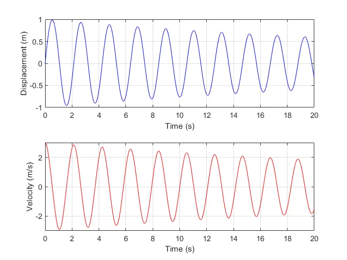
1) We could see that both the values of position and velocity tends to zero as time increases, mainly because of acceleration due to gravity which acts in a vertically downward direction. The plot matches with the real life scenario.

2) The velocity (magnitude) of the ball is maximum when it is at the bottom most position (i.e) when displacement = 0, and similarly the angular velocity is 0 when the ball reaches the highest point (maximum displacement magnitude).