Curve Fitting using MATLAB
Aim:
To write a code to perform curve fitting using MATLAB
Objectives:
1) Create linear and cubic fits and compare the goodness parameters of each fit for the given dataset (Temperature, Specific heat).
2) Perform splitwise operation to improve the fitness characteristics.
Theory:
Curve fitting is the process of constructing a curve, or mathematical function, that has the best fit to a series of data points, possibly subject to constraints. Curve fitting can involve either interpolation, where an exact fit to the data is required, or smoothing, in which a "smooth" function is constructed that approximately fits the data.
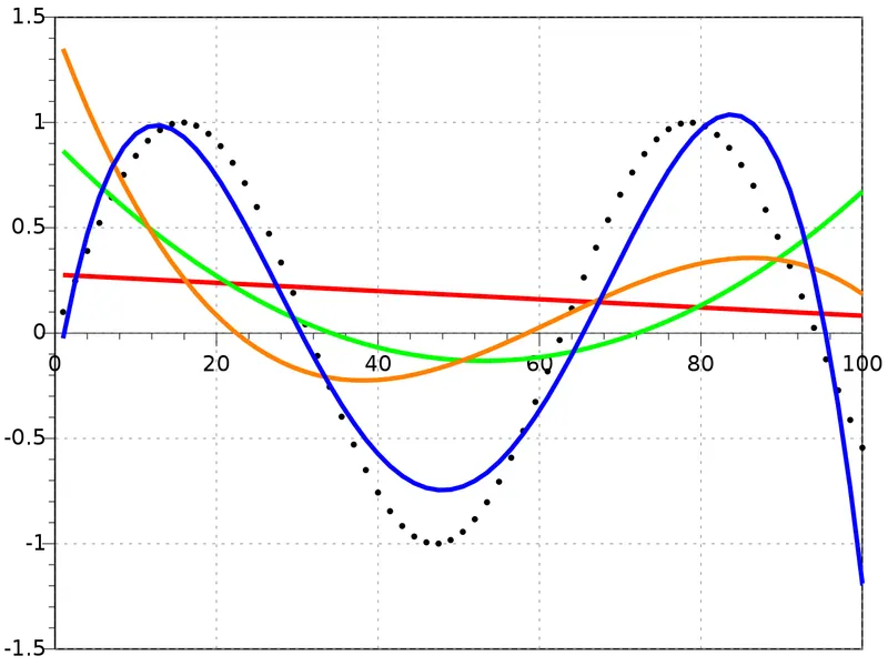
Polynomial curves fitting points generated with a sine function. The black dotted line is the "true" data, the red line is a first degree polynomial, the green line is second degree, the orange line is third degree and the blue line is fourth degree. The higher the order of function, the greater the accuracy.
Curve fitting is used to predict the population of a country, or stocks of a company of upcoming years, given the necessary inputs (factors that the event depends on). Even global warming can be predicted which helps a lot in putting a check to all the factors that contribute to the hike in temperature.
Goodness of a curve fit:
Parameters that helps us determine the goodness of the curve fit:
1) Sum of Squares due to Error (SSE)
`"Error" = |y(i)-"value of "f(x) " at " x(i)| = |y(i)-f(x(i))|`
SSE = `sum_(i=1) ^n ("Error"(i))^2`
Leeser the value of error, lesser the value of SSE, which ultimately leads to better curve fitting.
2) R-Square
`R^2=(SSR)/(SST)`
SSR - Sum of Squares of regression
`SSR = sum_(i=1) ^n (f(x(i))-Mean)^2`
SST = SSE + SSR
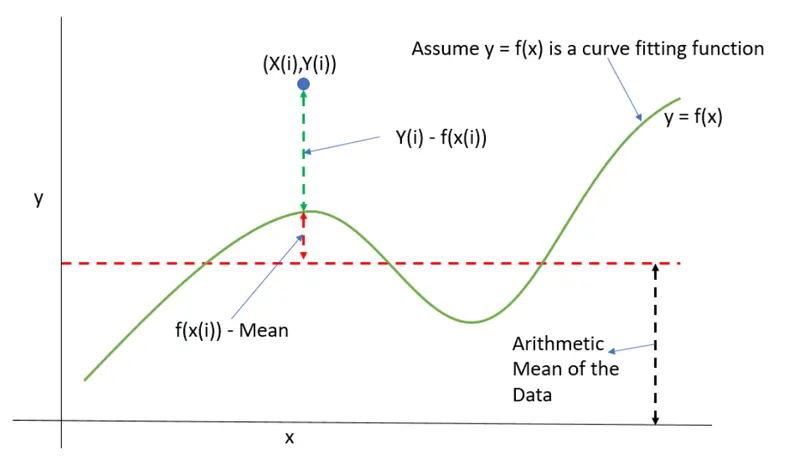
R Square is the ratio of SSR and SST which are mentioned above, where SSR is a part of SST. Therefore the values of `R^2` always lies within 0 - 1. The value of `R^2` that nearly tends to 1 gives a good curve fit. Usually `R^2>0.95` is considered a good curve fit.
3) Adjusted R-Square
Unlike R Square method, adjusted R Square only takes into account the values upon which the given function is dependent on (i.e) it ignores the variables that in no way affects the final outcome result.
`R_(adj)^2 = 1-((1-R^2)xx(n-1))/(n-k-1)`
n - number of data points
k - number of independent variables
Therefore as the value of k increases, the adjusted R-Square will decrease and vice versa.
4) Root Mean Squared Error
`RMSE = sqrt((SSE)/n)`
The RMSE represents the square root of the second sample moment of the differences between predicted values and observed values or the quadratic mean of these differences. These deviations are called residuals when the calculations are performed over the data sample that was used for estimation and are called errors (or prediction errors) when computed out-of-sample. The RMSE serves to aggregate the magnitudes of the errors in predictions for various data points into a single measure of predictive power. RMSE is a measure of accuracy, to compare forecasting errors of different models for a particular dataset and not between datasets, as it is scale-dependent.
It is a non-negative, and a value of 0 would indicate a perfect fit to the data (almost never achieved in practice).
MATLAB code:
1) Linear and Cubic Curve Fit
% Curve Fit
clear all
close all
clc

% Preparing the data
cp_data = load('data');              % loads the file name 'data' stored
temperature = cp_data(:,1);          % retrieves Temperature values
cp = cp_data(:,2);                   % retrieves Specific Heat values

% coefficients = polyfit(x,y,order of expression)
% Linear fit
co_effs1 = polyfit(temperature,cp,1);               % Calculating coefficients for linear equation
predicted_cp_1 = polyval(co_effs1,temperature);     % Calculating predicted values of specific heat

% Cubic fit
co_effs2 = polyfit(temperature,cp,3);               % Calculating coefficients for cubic equation
predicted_cp_3 = polyval(co_effs2,temperature);     % Calculating predicted values of specific heat

% Compare curve fit with the original data
plot(temperature,cp,'linewidth',2)                         % Original dataset
hold on;
plot(temperature,predicted_cp_1,'r','linewidth',3)         % Predicted linear ploynomial fit
plot(temperature,predicted_cp_3,'g','linewidth',3)         % Predicted cubic polynomial fit
xlabel('Temperature [K]')
ylabel('Specific heat [kJ/kmol-K]')
legend('Original dataset','Linear fit','Cubic fit')

% Evaluation of goodness of fit for linear fit
    m = mean(cp);       % Mean of specific heats
    n = length(cp);     % Number of data points
    k = 1;              % Number of independent variable (Temperature)

    % SSE (Sum of Square of Error)
    SSE1 = sum((cp-predicted_cp_1).^2);

    % R Square
    % SSR (Sum of Squares of Regression)
    SSR1 = sum((predicted_cp_1-m).^2);
    SST1 = SSE1 + SSR1;
    R1 = SSR1/SST1;

    % Adjusted R Square
    R_adj1 = 1 - ((1-R1)*(n-1)/(n-k-1));

    % RMSE (Root Mean Squared Error)
    RMSE1 = sqrt(SSE1/n);

% Evaluation of goodness of fit for cubic fit

    % SSE (Sum of Square of Error)
    SSE2 = sum((cp - predicted_cp_3).^2);

    % R Square
    % SSR (Sum of Squares of Regression)
    SSR2 = sum((predicted_cp_3 - m).^2);
    SST2 = SSE2 + SSR2;
    R2 = SSR2 / SST2;

    % Adjusted R Square
    R_adj2 = 1 - ((1 - R2)*(n - 1)/(n - k - 1));

    % RMSE (Root Mean Squared Error)
    RMSE2 = sqrt(SSE2 / n);

Linear_Fit_Evaluation = [SSE1;R1;R_adj1;RMSE1];
Cubic_Fit_Evaluation = [SSE2;R2;R_adj2;RMSE2];
Eval = {'Sum of Square due to error';'R Square';'Adjusted R square';'Root Mean Squared Error'};  % Row names
Goodness_Parameters = table(Linear_Fit_Evaluation,Cubic_Fit_Evaluation,'RowNames',Eval)          % Displaying Goodness paramaeters
Explanation:
i) Data of Temperature and Specific heat is retrieved from the system.
ii) Calculate the coefficients a,b of the equation `ax+b` for linear curve fit and a,b,c,d of the equation `ax^3+bx^2+cx+d` for cubic curve fit using the 'polyfit' command. Store coeficients in a new variable 'co_effs' (seperate for linear and cubic).
iii) Use the coefficients of the polynomial to predict the values of the function y(x) (i.e) Specific heat, using the 'polyval' command.
iv) After obtaining the values of the specific heat, plot the original data and the predicted data in order to comapre the results.
v) The aforementioned goodness parameters Sum of Squares of Error, R-Square, Adjusted R-Square, Root Mean Squared Error are calculated for the predicted data.
vi) Compare the results of the Linear and Cubic curve fit and propose which one serves a better result.
Results:
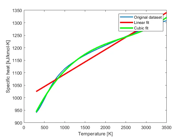
Fig 1: Plot displaying the original dataset, linear fit and cubic curve fit.
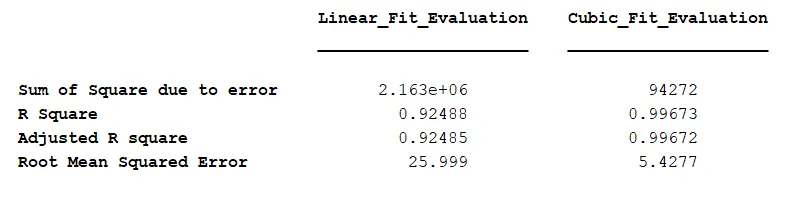
Fig 2: Manually calculated goodness parameters using the Matlab code.
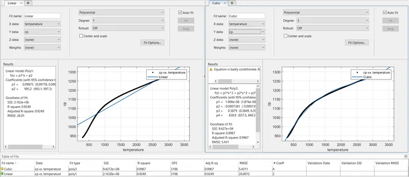
Fig 3: Goodness parameters using Curve Fitting Toolbox
Inference:
i) We could see that the goodness parameters for cubic curve is a better fit than the linear curve since it has a lesser SSE, RMSE value and a higher R-Square, Adjusted R-Square value.
ii) Althogh it seems to be a better fit, we get the warning as the equation is badly conditioned, (i.e) for any value outside the dataset, the predicted value might have a drastic difference to that of the observed value which is not a good characteristic. In order to avoid this, we use the splitwise method.
2) Splitwise method
% Splitwise Curve Fit
clear all
close all
clc

% Preparing the data
cp_data = load('data');              % loads the file name 'data' stored

temperature = cp_data(:,1);          % retrieves Temperature values
cp = cp_data(:,2);                   % retrieves Specific Heat values

% Splitting the data to 5 equal parts
temp1 = temperature(1:640);
cp1 = cp(1:640);
temp2 = temperature(641:1280);
cp2 = cp(641:1280);
temp3 = temperature(1281:1920);
cp3 = cp(1281:1920);
temp4 = temperature(1921:2560);
cp4 = cp(1921:2560);
temp5 = temperature(2561:3200);
cp5 = cp(2561:3200);

% coefficients = polyfit(x,y,order of expression)
% predicted value = polyval(coefficients,x)

co_effs1 = polyfit(temp1,cp1,1);                    % Calculating coefficients 0f 1st dataset
predicted_cp(:,1) = polyval(co_effs1,temp1);        % Calculating predicted values of specific heat for 1st dataset

co_effs2 = polyfit(temp2,cp2,1);                    % Calculating coefficients 0f 2nd dataset
predicted_cp(:,2) = polyval(co_effs2,temp2);        % Calculating predicted values of specific heat for 2nd dataset

co_effs3 = polyfit(temp3,cp3,1);                    % Calculating coefficients 0f 3rd dataset
predicted_cp(:,3) = polyval(co_effs3,temp3);        % Calculating predicted values of specific heat for 3rd dataset

co_effs4 = polyfit(temp4,cp4,1);                    % Calculating coefficients 0f 4th dataset
predicted_cp(:,4) = polyval(co_effs4,temp4);        % Calculating predicted values of specific heat for 4th dataset

co_effs5 = polyfit(temp5,cp5,1);                    % Calculating coefficients 0f 5th dataset
predicted_cp(:,5) = polyval(co_effs5,temp5);        % Calculating predicted values of specific heat for 5th dataset

% Compare curve fit with the original data
plot(temperature,cp,'g','linewidth',5)                  % Original dataset
hold on;
plot(temp1,predicted_cp(:,1),'r','linewidth',2)         % Predicted ploynomial fit for 1st dataset
plot(temp2,predicted_cp(:,2),'r','linewidth',2)         % Predicted ploynomial fit for 2nd dataset
plot(temp3,predicted_cp(:,3),'r','linewidth',2)         % Predicted ploynomial fit for 3rd dataset
plot(temp4,predicted_cp(:,4),'r','linewidth',2)         % Predicted ploynomial fit for 4th dataset
plot(temp5,predicted_cp(:,5),'r','linewidth',2)         % Predicted ploynomial fit for 5th dataset

xlabel('Temperature [K]')
ylabel('Specific heat [kJ/kmol-K]')
legend('Original dataset','Curve fit')

for i=1:5
    % Evaluation of goodness of fit for linear fit
    m(i) = mean(cp(((i-1)*640)+1:i*640));        % Mean of specific heats for each set
    n = length(cp)/5;                            % Number of data points
    k = 1;                                       % Number of independent variable (Temperature)

    % SSE (Sum of Square of Error)
    SSE(i) = sum((cp(((i-1)*640)+1:i*640)-predicted_cp(:,i)).^2);

    % R Square
    % SSR (Sum of Squares of Regression)
    SSR(i) = sum((predicted_cp(:,i)-m(i)).^2);
    SST(i) = SSE(i) + SSR(i);
    R(i) = SSR(i)/SST(i);

    % Adjusted R Square
    R_adj(i) = 1 - ((1-R(i))*(n-1)/(n-k-1));

    % RMSE (Root Mean Squared Error)
    RMSE(i) = sqrt(SSE(i)/n);
end

SSE_final = mean(SSE);
R_Square = mean(R);
R_adj_final = mean(R_adj);
RMSE_final = mean(RMSE);

Splitwise_Fit_Evaluation = [SSE_final;R_Square;R_adj_final;RMSE_final];
Eval = {'Sum of Square due to error';'R Square';'Adjusted R square';'Root Mean Squared Error'};     % Row names
Goodness_Parameters = table(Splitwise_Fit_Evaluation,'RowNames',Eval)                               % Displaying Goodness paramaeters
Explanation:
1) In the case of splitwise method, the exact same steps are followed except for the part where the inital dataset is divided equally into 5 parts.
2) Each part undergoes the same steps as we found for linear curve fit.
3) Finally to calculate the goodness parameters of the given data, they are calculated individually for each dataset and the average value is found.
Results:
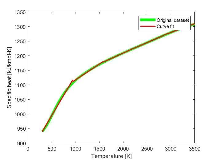
Fig 4: Plot comparison between original data and splitwise curve fit
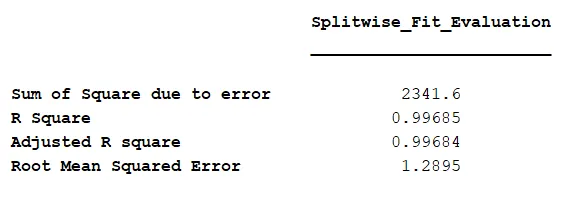
Fig 5: Goodness parameter values using splitwise method
Inference:
1) Using splitwise method, we get the R-Square value of 0.99685 which is greater than 0.92488 which was obtained for linear curve fit by normal procedure. This proves that using splitwise operation, we could yield better curve fits which may deviate lesser from the given data when a point is provided outside the given dataset.
2) Also a much lower SSE and RMSE value shows that the splitwise method is more efficient to get a better fit.
Questions:
1) How to make a curve fit perfectly?
Perfect curve fit is the fit that exactly matches with the given data at each and every data point. It is practically not possible to attain a perfect fit, but there are methods to attain the nearest answer possible without any imbalance in the equation. Among many curve fitting methods, Interpolant method proves to be the best way to get the closest results. While using polynomial curve fitting to get the perfect fit, it is necessary to make sure that the equation isn't imbalanced. In case if it is imbalanced, even though the resulting curve fit may seem to fit the original data perfectly, it becomes absolutely erroneous for a point outside the given dataset.
2) How to get the best fit?
Best fit refers to a line through a scatter plot of data points that best expresses the relationship between those points. Statisticians typically use the least squares method to arrive at the geometric equation for the line. A straight line will result from a simple linear regression analysis of two or more independent variables. A regression involving multiple related variables can produce a curved line in some cases.
To perform a regression analysis, collect a set of data points, each including a complete set of dependent and independent variables.
On a chart, these data points would appear as scatter plot, a set of points that may or may not appear to be organized along any line. If a linear pattern is apparent, it may be possible to sketch a line of best fit that minimizes the distance of those points from that line. If no organizing axis is visually apparent, regression analysis can generate a line based on the least squares method. This method builds the line which minimizes the squared distance of each point from the line of best fit.
3) What could be done to improve the cubic fit?
The cubic fit can be improved by using the splitwise operation mentioned above. This splits the given data into various parts and then performing the task to each set individually thus reducing the overall error. This is evident from the goodness parameter values obtained from both the methods proving that splitwise method yeilds a much more efficient fit.
References
1) https://in.mathworks.com/help/curvefit/fit-comparison-in-curve-fitting-app.html
2) https://www.investopedia.com