Genetic Algorithm Optimization using MATLAB

Aim:

To write a code to find global maxima using MATLAB.

Objectives:

1) Optimize the user defined stalagmite function and find the global maxima using the Genetic Algorithm command.

2) Bring out the same final answer irrespective of the number of times the code is executed, since Genetic Algorithm command picks up random initial values for every trial (it is necessary to optimise the function efficiently).

Theory:

Genetic Algorithm (ga):

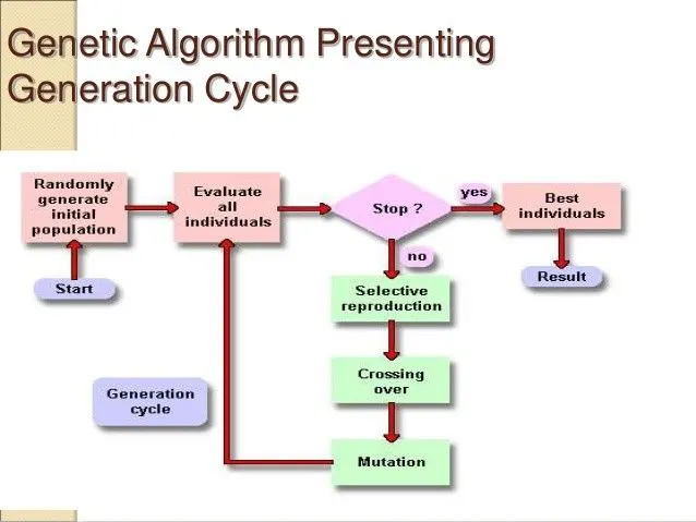
It is an optimization technique used to solve non-linear or non-differentiable optimization problems. It works by starting with initial generation of candidate solutions that are tested against the objective function. The subsequent generations evolve from the first generation through (i) Selection (ii) Crossover (iii) Mutation. Incase we have a function with 2 local minima and 1 global minima. Initially it randomly picks up a set of points and evaluates them to determine the fitness function. It then selects few good solutions that lie near the minimas as parents to continue to the next generation. Subsequent population for iteration 2 is evaluated using selection, crossover and mutation, using the parent values obtained from previous iteration. This process is continued until the algorithm converges. The algorithm converges based on different criteria, which is later discussed in the project.

Creation of Next Generation:

The genetic algorithm uses the current population to create the children that make up the next generation. The algorithm selects a group of individuals in the current population, called parents, who contribute their genes (the entries of their vectors) to their children. The algorithm usually selects individuals that have better fitness values as parents.

The genetic algorithm creates three types of children for the next generation:

• Elite : The individuals in the current generation with the best fitness values. These individuals automatically survive to the next generation.
• Crossover : Created by combining the vectors of a pair of parents. Selects the common similarities from the parent variables and retains them for children variables.
• Mutation children : Created by introducing random changes, or mutations, to a single parent. It allows the genetic algorithm to avoid falling into the local minima and helps to explore the solution space.

Stopping (convergence) Criteria:

The aforementioned generation process continues as long as it meets the convergence criteria. Some of the popular convergence criteria are (i) Specifying a maximum limit to the number of generations created (ii) When change in fitness function values is negligible.

The following options are some important option commands to determine when to stop:

• MaxGenerations — The algorithm stops when the number of generations reaches MaxGenerations.
• MaxStallGenerations — The algorithm stops when the average relative change in the fitness function value over MaxStallGenerations is less than Function tolerance.
• FunctionTolerance — The algorithm runs until the average relative change in the fitness function value over MaxStallGenerations is less than Function tolerance.

ga Syntax:

x = ga(fun,nvars,A,b,Aeq,beq,lb,ub,nonlcon,options)

1. fun - Objective function, specified as a function handle or function name. Write the objective function to accept a row vector of length nvars and return a scalar value.
2. nvars - Number of variables, specified as a positive integer. The solver passes row vectors of length nvars to fun
3. A - Linear inequality constraints, specified as a real matrix. A is an M-by-nvars matrix, where M is the number of inequalities. It consists of the coefficients of the variables from the LHS.
4. b - Linear inequality constraints, specified as a real vector. b is an M-element vector related to the A matrix. It consists of the values from the RHS of the given linear equations.
5. Aeq - Linear equality constraints, specified as a real matrix. Similar to A, but without any inequality in the equations.
6. beq - Linear equality constraints, specified as a real matrix. Similar to b, but without any inequality in the equations.
7. lb - lb represents the lower bounds element-wise in lb ≤ x ≤ ub.
8. ub - ub represents the upper bounds element-wise in lb ≤ x ≤ ub.
9. nonlcon - Nonlinear constraints, specified as a function handle or function name. nonlcon is a function that accepts a vector or array x and returns two arrays, c(x) and ceq(x).

   c(x) is the array of nonlinear inequality constraints at x. ga attempts to satisfy c(x) <= 0 for all entries of c.

   ceq(x) is the array of nonlinear equality constraints at x. ga attempts to satisfy ceq(x) = 0 for all entries of ceq.

10. options - Optimization options, specified as the output of optimoptions or a structure. Various operating conditions can be specified in options including some of the commands we discussed earlier - InitialPopulationRange, MaxStallTime, MaxStallGenerations, PopulationSize, SelectionFcn, FitnessLimit, FunctionTolerance.

Stalagmite Function:

`f(x,y) = f_(1,x)f_(2,x)f_(1,y)f_(2,y)`

where

`f_(1,x)=[sin(5.1pix+0.5)]^6`

`f_(1,y)=[sin(5.1piy+0.5)]^6`

`f_(2,x)=exp[-4xxln(2)((x-0.0667)^2)/0.64]`

`f_(2,y)=exp[-4xxln(2)((y-0.0667)^2)/0.64]`

MATLAB Code:

Stalagmite function:

function [f] = stalagmite(input_vector)
x = input_vector(1);
y = input_vector(2);
f_1x = (sin((5.1*pi*x)+0.5))^6;
f_1y = (sin((5.1*pi*y)+0.5))^6;
f_2x = exp(-4*log(2)*((x-0.06667)^2)/0.64);
f_2y = exp(-4*log(2)*((y-0.06667)^2)/0.64);
f = -f_1x*f_2x*f_1y*f_2y;
end

Explanation:

1. The function calculates the value f for the point x and y which are sent as parameters.
2. The ga function finds the global minima and we are supposed to find the global maxima for the given problem statement. Therefore we multiply with a negative sign in order to find the minima.
3. The variable f stores the final value of the function.

Genetic Algorithm - Study 1 :

clear all
close all
clc

% Defining our search space
x = linspace(0,0.6,150);
y = linspace(0,0.6,150);
% Number of iterations
num_cases = 50;

% Creating a 2 Dimensional mesh
[xx,yy] = meshgrid(x,y);

% Evaluating stalagmite function
for i=1:length(xx)
    for j=1:length(yy)
        input_vector(1) = xx(i,j);
        input_vector(2) = yy(i,j);
        f(i,j) = stalagmite(input_vector);
    end
end

% Study 1 - Statistical Behaviour
tic
for i=1:num_cases
        % Storing the maximum value of f and the corresponding x, y values at each iteration
        [inputs,fval(i)] = ga(@stalagmite,2);
        x1(i) = inputs(1);
        y1(i) = inputs(2);
end
figure(1)
subplot(2,1,1)
surfc(xx,yy,f);                 % Plots the surface with function values at each grid point
xlabel('x value')
ylabel('y value')
zlabel('f value')
shading interp                  % Hides the mesh lines
hold on
plot3(x1,y1,fval,'marker','o','markersize',5,'markerfacecolor','r')     % Plots the maximum value obtained during every iteration process
title('Unbounded inputs')
subplot(2,1,2)
plot(fval)
xlabel('Iterations')
ylabel('Function minimum')
study1_time = toc;              % Evaluating the time taken to converge

Explanation:

1. First we initialize the search space x, y and the number of iterations. The main reason for providing the number of iterations to check whether we get the same global maxima value after every iteration.
2. Then we create the grid plot with x, y values using the meshgrid command.
3. Every single coordinate in the grid plot is fed to the user defined stalagmite function which returns the values of the function which is stored in a 2D array. Since we have considered x, y as an integer in stalagmite function, each coordinate is sent seperately using nested for-loop.
4. The ga function returns the maximum function value and the corresponding x, y coordinates which is then stored in an array.
5. In study 1, the parameters sent are just the function and the number of variables. Even though the search space is defined, ga is a random-based classical evolutionary algorithm, therefore it selects random sample space during each iteration.
6. The stalagmite function value for each coordinate is plotted using the surfc command.
7. In order to showcase the variation in the minima value in every iteration, the global maxima for each iteration is plotted seperately in the plot window 2.
8. The tic toc command is used to determine the time taken to evaluate the entire program.

Results:

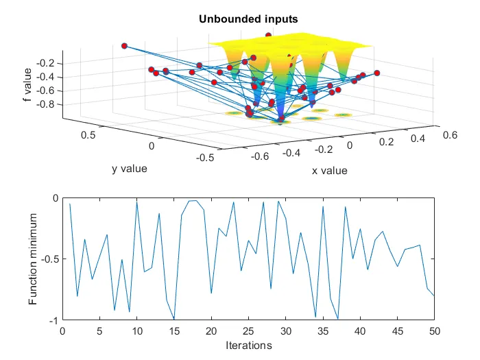
Fig 1: (i) Plot showing the global and local minima values for study 1 (ii) Minima value during each iteration

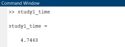
Fig 2: Time taken for compiling study 1

Inference:

1. We could see that the ga function has taken population out of the seach space. This is because no boundary limits were specified explicitly in the ga command.
2. The variation in the global minima value is clear seen in plot 2.
3. We could see that this study yielded the correct results only during 3 iterations (15, 34, 37).

Genetic Algorithm - Study 2:

It is similar to study 1 except for the fact that the lower bounds (lb) and upper bounds (ub) are specified in the ga command.

clear all
close all
clc

% Defining our search space
x = linspace(0,0.6,150);
y = linspace(0,0.6,150);
% Number of iterations
num_cases = 50;

% Creating a 2 Dimensional mesh
[xx,yy] = meshgrid(x,y);

% Evaluating stalagmite function
for i=1:length(xx)
    for j=1:length(yy)
        input_vector(1) = xx(i,j);
        input_vector(2) = yy(i,j);
        f(i,j) = stalagmite(input_vector);
    end
end

% Study 2 - Statistical Behaviour with upper and lower bounds
tic
for i=1:num_cases
        % Storing the maximum value of f and the corresponding x, y values at each iteration
        [inputs,fval(i)] = ga(@stalagmite,2,[],[],[],[],[0;0],[0.6;0.6]);
        x1(i) = inputs(1);
        y1(i) = inputs(2);
end
figure(2)
subplot(2,1,1)
surfc(xx,yy,f);                 % Plots the surface with function values at each grid point
xlabel('x value')
ylabel('y value')
zlabel('f value')
shading interp                  % hides the mesh lines
hold on
plot3(x1,y1,fval,'marker','o','markersize',5,'markerfacecolor','r')     % Plots the maximum value obtained during every iteration process
title('Bounded inputs')
subplot(2,1,2)
plot(fval)
xlabel('Iterations')
ylabel('Function minimum')
axis([0,num_cases,-1.1,-0.6])
study2_time = toc;             % Evaluating the time taken to converge

Results:

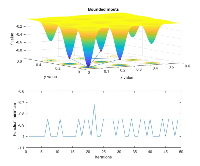
Fig 3: (i) Plot showing the global and local minima values for study 2 (ii) Minima value during each iteration

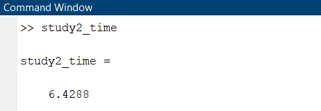
Fig 4: Time taken for compiling study 2

Inference:

1. We could still see variation in results in different iterations, but it is also clear that it varies only among 4 points (i.e) the global maxima and 3 other local maxima. This result is much better when comapred to the results from the previous study.
2. Since we have specified the upper and lower boundary values, the ga function only takes population values from the given range.
3. We could also see an increase in the compuation time.

Genetic Algorithm - Study 3:

Similar to study 2, only chane is to explicitly set the population size to 170, which previous had a default value of 50.

clear all
close all
clc

% Defining our search space
x = linspace(0,0.6,150);
y = linspace(0,0.6,150);
% Number of iterations
num_cases = 50;

% Creating a 2 Dimensional mesh
[xx,yy] = meshgrid(x,y);

% Evaluating stalagmite function
for i=1:length(xx)
    for j=1:length(yy)
        input_vector(1) = xx(i,j);
        input_vector(2) = yy(i,j);
        f(i,j) = stalagmite(input_vector);
    end
end

% Study 3 - increasing the number of GA iterations
tic
options = optimoptions('ga','PopulationSize',170);
for i=1:num_cases
        % Storing the maximum value of f and the corresponding x, y values at each iteration
        [inputs,fval(i)] = ga(@stalagmite,2,[],[],[],[],[0;0],[0.1;0.1],[],[],options);
        x1(i) = inputs(1);
        y1(i) = inputs(2);
end
figure(3)
subplot(2,1,1)
surfc(xx,yy,f);                  % Plots the surface with function values at each grid point
xlabel('x value')
ylabel('y value')
zlabel('f value')
shading interp                   % hides the mesh lines
hold on
plot3(x1,y1,fval,'marker','o','markersize',5,'markerfacecolor','r')     % Plots the maximum value obtained during every iteration process
title('Bounded inputs with increased population size')
subplot(2,1,2)
plot(fval)
axis([0,num_cases,-1.1,-0.9])
xlabel('Iterations')
ylabel('Function minimum')
study3_time = toc;               % Evaluating the time taken to converge

Results:

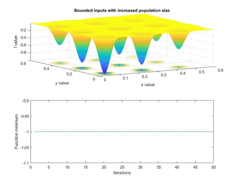
Fig 5: (i) Plot showing the global minima value for study 3 (ii) Minima value during each iteration

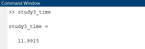
Fig 6: Time taken for compiling study 3

Inference:

1. Increase in the population size using the optimoptions command gives a much better result for global maxima when comared to study 2.
2. From the previous studies, we learnt that the actual global maxima value is approimately tending to be 1. Therefore we confine the upper and lower bounds nearing to the x, y coordinates of the global maxima.
3. Increase in population size also means that increase in number of expressions to be evaluated which eventually leads to increase in computation time.
4. After optimizing the ga function efficiently, we get 1 constant value for all 50 iterations.

Reference:

1) https://in.mathworks.com/help

2) https://in.mathworks.com/help/gads/ga

3) https://en.wikipedia.org/wiki/Genetic_algorithm

4) https://in.mathworks.com/discovery/genetic-algorithm.html