Rankine Cycle Simulator using MATLAB
Aim:
To write a code to plot the Rankine cycle and to calculate the thermal efficiency of the cycle.
Objectives:
1) Collect the required inputs of temperature and pressure from the user
2) Substitute these values in the formulas to calculate the work done and the thermal efficiency of the cycle
3) Plot the results using T-S and H-S diagram
Theory:
Rankine cycle consists of 4 main components:
i) Pump
ii) Boiler
iii) Turbine
iv) Condenser
Pump is used to compress the steam (in liquid form) which is obtained from the conderser. A pump is used in the case of rankine cycle because, it consumes less power when compared to compressor. Since the steam in the previous state is completely transformed to liquid, a pump is sufficient to compress liquid, which would have not been the case if the fluid was a mixture of liquid and vapour (in which case a compressor must be used). Boiler is used to raise the temperature of the fluid to the required amount so that the phase change of liquid to vapour state takes place. Turbine is the main component which provides the work, which can be later transformed to any form of energy according to the needs. Condenser is used to reduce the temperature of steam which allows it to go through the phase change from gas to liquid.
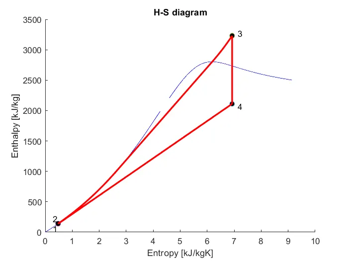
Process 1->2 Isentropic compression in Pump
Process 2->3 Constant pressure heat addition in Boiler
Process 3->4 Isentropic expansion in Turbine
Process 4->1 Constant pressure heat rejection in Condenser
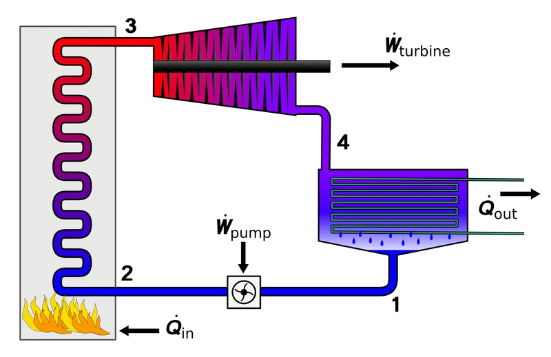
The Rankine cycle is a model used to predict the performance of steam turbine systems. It was also used to study the performance of reciprocating steam engines. The Rankine cycle is an idealized thermodynamic cycle of a heat engine that converts heat into mechanical work while undergoing phase change. It is an idealized cycle in which friction losses in each of the four components are neglected. The heat is supplied externally to a closed loop, which usually uses water as the working fluid.
In an ideal Rankine cycle the pump and turbine would be isentropic, i.e., the pump and turbine would generate no entropy and hence maximize the net work output. Processes 1–2 and 3–4 would be represented by vertical lines on the T–S diagram and more closely resemble that of the Carnot cycle. The Rankine cycle shown here prevents the state of the working fluid from ending up in the superheated vapor region after the expansion in the turbine, which reduces the energy removed by the condensers.
The actual vapor power cycle differs from the ideal Rankine cycle because of irreversibilities in the inherent components caused by fluid friction and heat loss to the surroundings; fluid friction causes pressure drops in the boiler, the condenser, and the piping between the components, and as a result the steam leaves the boiler at a lower pressure; heat loss reduces the net work output, thus heat addition to the steam in the boiler is required to maintain the same level of net work output.
Formula:
`eta_(thermal)=W_("net")/Q_("in")`
`W_("net") = W_t-W_p`
`eta_(thermal)` - Thermal Efficiency of cycle
`W_"net"` - Net Work Done
`W_t` - Work done by Turbine
`W_p` - Work given to Pump
`Q_"in"` - Heat supplied to Boiler
Matlab Code:
clear all;
close all;
clc;

fprintf('                         Rankine cycle Simulatornn');
disp('Process 1->2 Isentropic compression in Pump')
disp('Process 2->3 Constant pressure heat addition in Boiler')
disp('Process 3->4 Isentropic expansion in Turbine')
disp('Process 4->1 Constant pressure heat rejection in Condenser')
fprintf('n')

p3 = input('Enter the pressure at the inlet of the Turbine (bar):  ');
t3 = input('Enter the temperature at the inlet of the Turbine (°C):  ');
p4 = input('Enter the pressure at the inlet of the Condenser (bar):  ');

p2 = p3; % Process 2->3 constant pressure process
p1 = p4; % Process 4->1 constant pressure process

%State 3
h3 = XSteam('h_pT',p3,t3);
s3 = XSteam('s_pT',p3,t3);

% state 4
s4 = s3;
h4 = XSteam('h_ps',p4,s4);
t4 = XSteam('T_ph',p4,h4);

%{
sf4 = XSteam('sL_p',p4);
sg4 = XSteam('sV_p',p4);
x4 = (s4-sf4)/(sg4 - sf4);
hf4 = XSteam('hL_p',p4);
hg4 = XSteam('hV_p',p4);
h4 = hf4 + x3*(hg4 - hf4);
%}

% state 1
h1 = XSteam('hL_p',p1);
v1 = XSteam('vL_p',p1);
s1 = XSteam('sL_p',p1);
t1 = t4;

% Work supplied to Pump
Wp = v1*100*(p2 - p1);

% State 2
h2 = h1 + Wp;
s2 = XSteam('s_ph',p2,h2);
t2 = XSteam('T_ph',p2,h2);

% Work done by Turbine
Wt = h3 - h4;

% Heat exchange at Condenser
Qout = h1 - h4;

% Heat exchange in Boiler
Qin = h3 - h2;

% Net Work output
W_net = Wt - Wp;

% Back Work Ratio
Wb = Wp/Wt;

% Thermal Efficiency
n = (W_net/Qin)*100;

% Saturation dome for H-S diagram
t_sat = linspace(0,374,500);
for i = 1:length(t_sat)
    h_sat1(i) = XSteam('hL_T',t_sat(i));
end

for i = 1:length(t_sat)
    h_sat2(i) = XSteam('hV_T',t_sat(i));
end

% Saturation dome for T-S diagram
for i = 1:length(t_sat)
    s_sat1(i) = XSteam('sL_T',t_sat(i));
end
for i = 1:length(t_sat)
    s_sat2(i) = XSteam('sV_T',t_sat(i));
end

% path for process 2->3 in T-S diagram
t_ad1 = linspace(t2,t3,50);
for i = 1:length(t_ad1)
    S1(i) = XSteam('s_pT',p2,t_ad1(i));
end

% path for process 2->3 in H-S diagram
S = linspace(s2,s3,100);
for i =1:length(S)
    H(i) = XSteam('h_ps',p2,S(i));
end

% Plotting H-S diagram
figure(1)
hold on;
plot(s_sat1,h_sat1,'b')
plot(s_sat2,h_sat2,'b')
plot(s1,h1,'o','MarkerSize',6,'MarkerFaceColor','k');
plot(s2,h2,'o','MarkerSize',6,'MarkerFaceColor','k');
plot(s3,h3,'o','MarkerSize',6,'MarkerFaceColor','k');
plot(s4,h4,'o','MarkerSize',6,'MarkerFaceColor','k');
text(s1-0.2,h1-80,'1');
text(s2-0.2,h2+80,'2');
text(s3+0.2,h3+40,'3');
text(s4+0.2,h4-40,'4');
line([s1,s2],[h1,h2],'linewidth',2,'color','r');
line([s3,s4],[h3,h4],'linewidth',2,'color','r');
line([s4,s1],[h4,h1],'linewidth',2,'color','r');
plot(S,H,'r','linewidth',2);
xlabel('Entropy [kJ/kgK]')
ylabel('Enthalpy [kJ/kg]')
title('H-S diagram')

% Plotting T-S diagram
figure(2)
hold on;
plot(s_sat1,t_sat,'b')
plot(s_sat2,t_sat,'b')
plot(s1,t1,'o','MarkerSize',6,'MarkerFaceColor','k');
plot(s2,t2,'o','MarkerSize',6,'MarkerFaceColor','k');
plot(s3,t3,'o','MarkerSize',6,'MarkerFaceColor','k');
plot(s4,t4,'o','MarkerSize',6,'MarkerFaceColor','k');
text(s1-0.2,t1-20,'1');
text(s2-0.2,t2+20,'2');
text(s3+0.2,t3+20,'3');
text(s4+0.2,t4-20,'4');
line([s1,s2],[t1,t2],'linewidth',2,'color','r');
line([s3,s4],[t3,t4],'linewidth',2,'color','r');
line([s4,s1],[t4,t1],'linewidth',2,'color','r');
plot(S1,t_ad1,'r','linewidth',2)
axis([0,10,0,500])
xlabel('Entropy [kJ/kgK]')
ylabel('Temperature [°C]')
title('T-S diagram')

% Displaying properties at each state point

fprintf('n')
disp('At state point 1:')
fprintf('P1 = %.3f kPan',p1)
fprintf('T1 = %.3f °Cn',t1)
fprintf('H1 = %.3f kJ/kgn',h1)
fprintf('S1 = %.3f kJ/kgKnn',s1)

disp('At state point 2:')
fprintf('P2 = %.3f kPan',p2)
fprintf('T2 = %.3f °Cn',t2)
fprintf('H2 = %.3f kJ/kgn',h2)
fprintf('S2 = %.3f kJ/kgKnn',s2)

disp('At state point 3:')
fprintf('P3 = %.3f kPan',p3)
fprintf('T3 = %.3f °Cn',t3)
fprintf('H3 = %.3f kJ/kgn',h3)
fprintf('S3 = %.3f kJ/kgKnn',s3)

disp('At state point 4:')
fprintf('P4 = %.3f kPan',p4)
fprintf('T4 = %.3f °Cn',t4)
fprintf('H4 = %.3f kJ/kgn',h4)
fprintf('S4 = %.3f kJ/kgKnn',s4)

fprintf('Work output Turbine (Wt) = %.3f kJ/kgn',Wt);
fprintf('Work input Pump (Wp) = %.3f kJ/kgn',Wp);
fprintf('Net Work done (Wnet) = %.3f kJ/kgn',W_net);
fprintf('Back work ratio (Wb) = %.3f kJ/kgn',Wb);
fprintf('Thermal Efficiency = %.3f%% n',n);
Explanation:
1) The pressure, temperature at the inlet of the turbine and the pressure at the inlet of the condenser is obtained from the user in the specified units.
2) XSteam function, which is previously stored in the same directory of the current program, calculates the property values given the conditions at that state point.
3) First law of Thermodynamics (Conservation of energy) is used to find the enthalpy and the entropy values at each state point provided the pressure, temperature.
4) A for loop is used to calculate the values of entropy and enthalpy in the saturation dome for T-S and H-S diagrams.
5) Since the process 2->3 follows a constant pressure during heat addition, the pressure at state point 2 is kept constant and the corresponding entropy values are found to draw the profile for the process.
6) Similarly the enthalpy profile is obtained in H-S diagram by keeping the pressure constant.
7) The work done by the turbine, net work done and thermal efficiency are found using the aforementioned formulas.
8) The graphs are plotted and the property values at each state point is displayed in the command window.
Output:
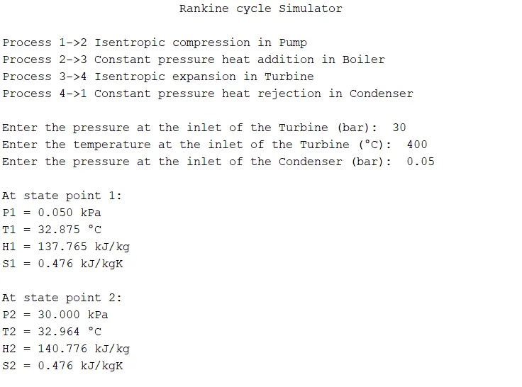
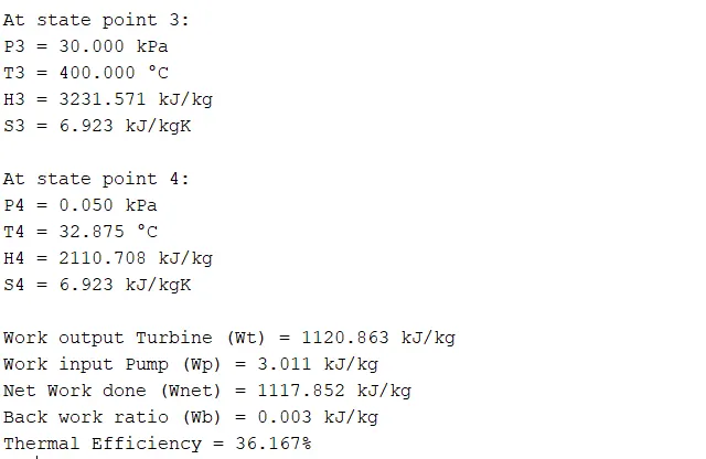
Plots:
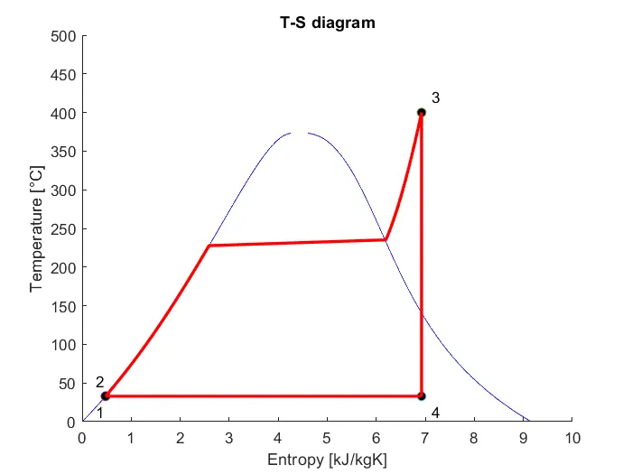
Inferenece:
1) In both the plots we could see that the points 1 and 2 are very close to each other implying that there is no significant change in temperature or enthalpy during the compression process in pump.
2) State point 4 in T-S diagram is far away from the vapour saturation line, this may lead to erosion. This can be prevented by reheating partial amount of vapour from the turbine.
3) It is also noticeable that the temperature and pressure remains constant within the saturation dome, which makes them non-independent variables and either pressure and volume or temperature and volume can be specified within the dome to calculate the properties at that point but pressure and temperature can not be provided as two independent properties.
4) In our case, since we have assumed 100% isentropic efficiencies, the entropies does not change during processes 1->2 and 3->4, which gives a vertical straight line in the T-S diagram.
Results:
The property values at each state points, work done, thermal efficiency and the plots for T-S and H-S diagrams are obtained.
References: