Week 2 Railwheel and Track
AIM:
Simulate the rail wheel and track for their lifecycle and the stress, strain, and total deformation provided by the wheel running on the track by the given forces
OBJECTIVE:
The objective of this challenge is to perform a static structural analysis on the Railwheel and Track setup and to Compare the Total Deformation, Equivalent stress, and the life under the two bearing loads such as 100000N and 500000N respectively. Also to implement a user-defined result calculate the Total Deformation from this result and to compare the Total Deformation obtained by the inbuilt result by ANSYS for a load of 100,000 N.
INTRODUCTION (THEORY)
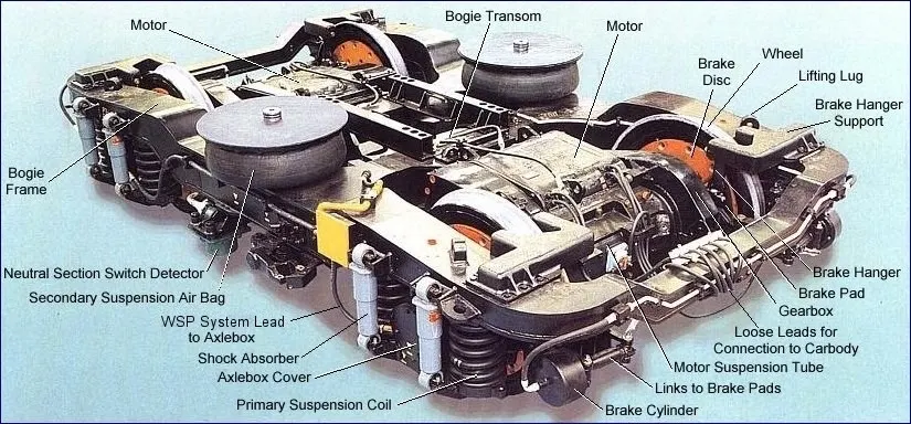
A train wheel or rail wheel is a type of wheel specially designed for use on railway tracks. A rolling component is typically pushed onto an axle and mounted directly on a railway carriage or locomotive, or
Indirectly on a bogie, also called a truck. Wheels are cast or forged and are heat-treated to have a specific hardness. New wheels are trued, using a lathe, to a specific profile before being pressed onto an axle. All-wheel profiles must be regularly checked to ensure proper interaction between the wheel and the rail. Incorrectly trued or worn-out wheels can increase rolling resistance, reduce energy efficiency, and even cause a derailment. A railroad wheel typically consists of two main parts: the wheel itself, and the tire (or tire in British English) around the outside. A rail tire is normally composed of steel, heated, and placed onto the wheel, where it stays securely in place throughout cooling and shrinking. While robust rail wheels feature a resilient substance, such as rubber, between the wheel and tire, monobloc wheels do not have surrounding tires.
Rail frequently experiences extremely high stresses and has a complicated stress zone where heat, contact, and bending forces are all acting simultaneously. Continuous rail wheel-to-rail wheel engagement has the side consequences of high frictional stress, high contact pressure, and ultimately wear. Wear changes how the wheel and rail interact, which changes the nature of the rolling contact fatigue rate and leads to shallow fracture propagation in the rails. Rolling Contact Fatigue, which results from wear on the rail or plastic material deformation, can hurt and produce surface fissures.
Wear-prone areas are indicated by material loss or plastic flow of metal. The high rail traffic, high contact pressures, unfavorable environmental conditions, etc.
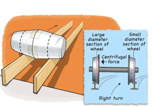
The wheels on each side of a train car are connected with a metal rod called an axle. This axle keeps the two train wheels moving together, both turning at the same speed when the train is moving.
This construction is great for straight tracks. But when a train needs to go around a bend the fact that both wheels are always rotating at the same rate can become a problem. The outside of a curve is slightly longer than the inside, so the wheel on the outside rail actually needs to cover more distance than the wheel on the inside rail. You can demonstrate this by drawing a train track—consisting of two rails—with a turn on a piece of paper. Take a measuring tape (or string and ruler) and measure the length of each line. The outside line of the track should be longer than the inside line. But how can one wheel cover more distance than the other one if they both are rotating at the same rate?
This is where the wheels' geometry comes in. To help the wheels stay on the track their shape is usually slightly conical. This means that the inside of the wheel has a larger circumference than the outside of the wheel. (They also have a flange, or raised edge, on the inner side to prevent the train from falling off the tracks.) When a train with slanted wheels turns, centrifugal force pushes the outside wheel to the larger part of the cone and pushes the inside wheel to the smaller part of the cone. As a result, when a train is turning it is momentarily running on wheels that are effectively two different sizes. As the outside wheel's circumference becomes larger it is able to travel a greater distance even though it rotates at the same rate as the smaller inside wheel. The train successfully stays on the tracks! In this activity, you will test for yourself how train wheel shapes impact their ability to stay on track.
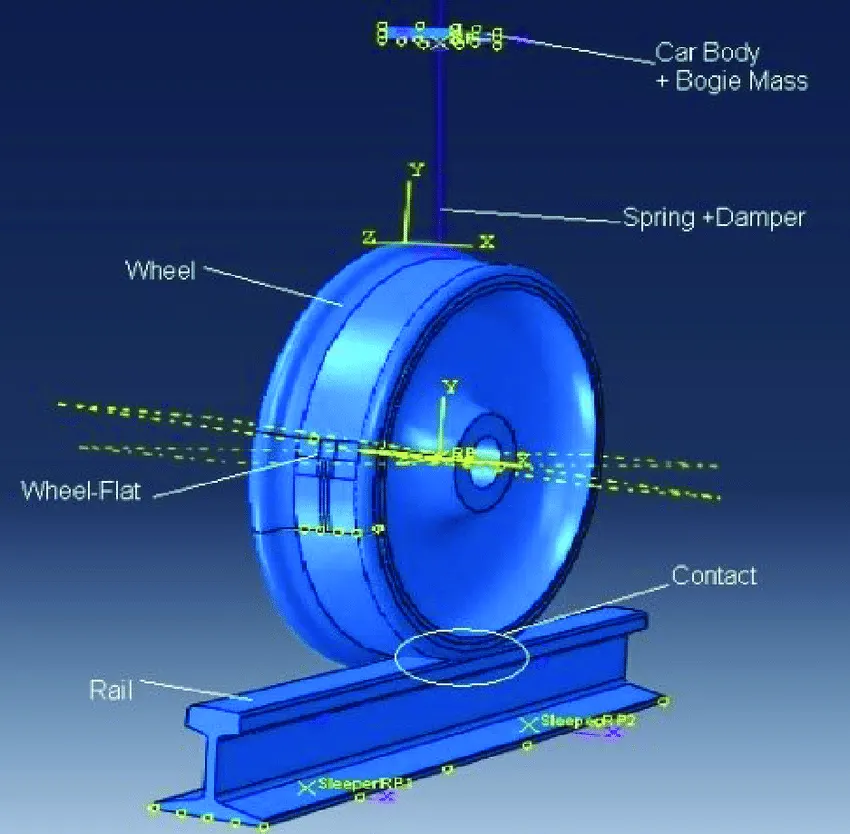
An image that depicts how ideally the tire and the track come into contact and all the terminologies associated with it.
Analysis Setup:
A static structural analysis will be conducted for a Railway wheel and Track mechanism for two different bearing load cases. Then a user-defined result is to be implemented to calculate the Total Deformation and verify it with the inbuilt result by ANSYS for a load of 100000 N.
- CASE 1: (Bearing Load at 100000 N)
- Geometry
The 3D assembly model of the Rail-wheel and track mechanism developed in SOLIDWORKS is shown in the figure below: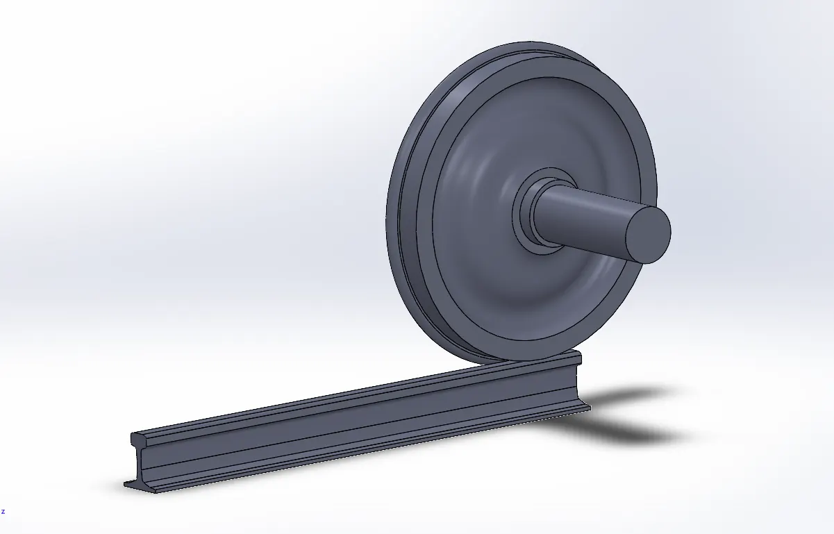
Material Properties
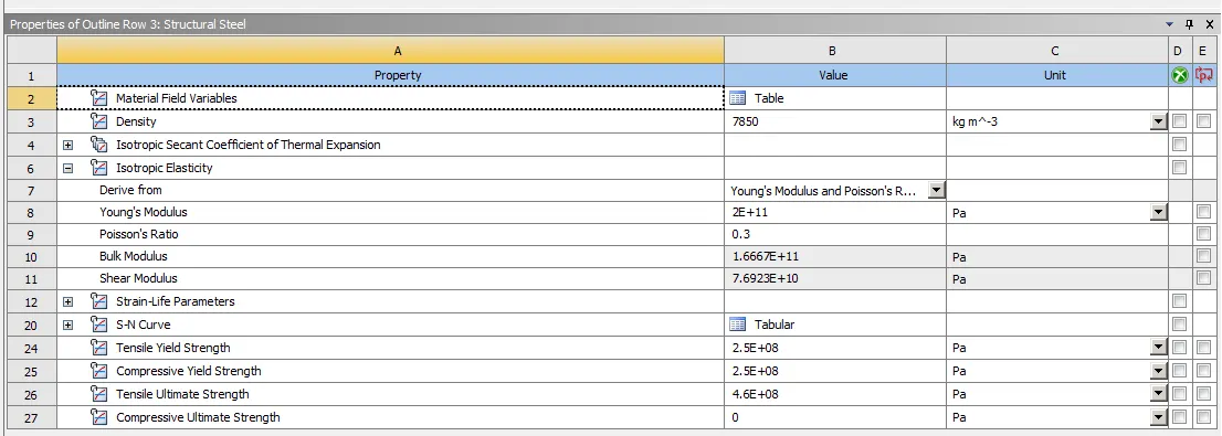
We applied structural steel material to do a static structural study on the rail, wheel, and track system; the material's mechanical characteristics are listed below:
Density : 7.85e-06 kg/mm³
Isotropic Secant Coefficient of Thermal Expansion: 1.2e-05 1/°C
Young's Modulus: 2e+05 MPa
Poisson's Ratio: 0.3
Bulk Modulus: 1.6667e+05 MPa
Shear Modulus: 76923 MPa
Tensile Yield strength: 250 MPa
Compressive Yield strength: 250 MPa
Tensile Ultimate strength: 460 MPa
Isotropic Thermal Conductivity: 0.0605 W/mm·°C
Specific Heat Constant Pressure: 4.34e+05 mJ/kg·°C
Contact Details
- Next step is to apply the Contacts to the geometry.
- To do so, expand the Contacts option present in the Connections menu.
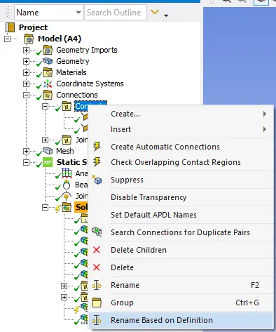
- First select both the Contact Regions then right-click and select Rename Based on Definition, as shown below:
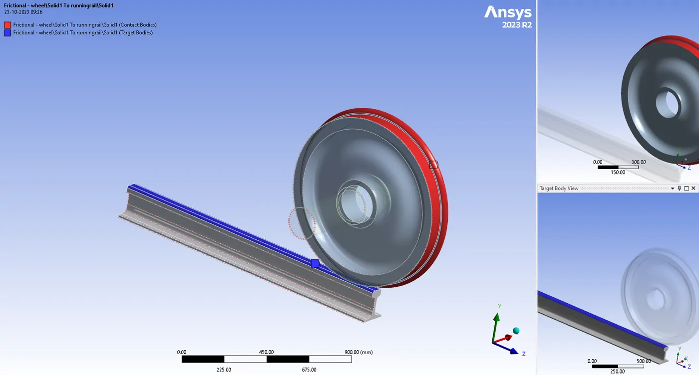
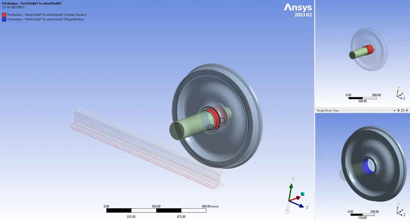
The wheel and the track and the wheel and the axle were designated as the two places in contact. The contact between the wheel and the running rail has a 0.3 coefficient of friction. As the rail is relatively flat and the wheel at the contact is convex, those two are chosen as the Contact Body and the Target Body, respectively. Initial frictionless contact between the wheel and the axle enables sliding without any loss of energy. Here, the wheel's rim is targeted while the axle's outside surface is made contact with. As a result, the contact body's surface is smaller than that of the target body.
- First contacts are created between the rail wheel and track by selecting the faces, the Contact type is frictional with a friction coefficient of 0.3
- Second contacts were created between the railwheel and shaft . The contact type is frictionless
Fix joint is deployed at track to avoid all types of movement that is all rotational and translational movement.
This joint is for the ground to running-rail, select both side of the track, the fixed joint connection type is body to ground
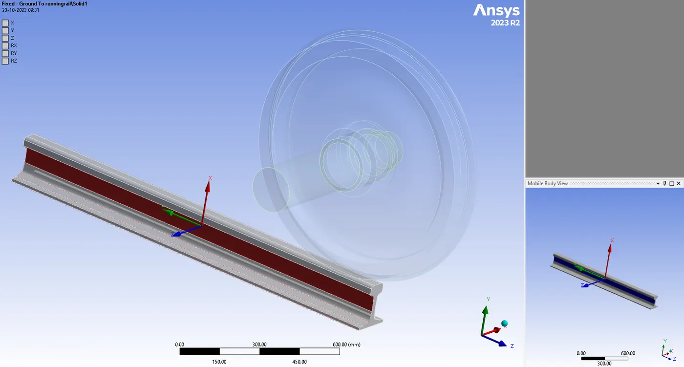
Now add a joint for the Shaft, such that the shaft can perform the translational motion along the Track. To do so, add another joint, then assign the Connection Type as Body-Ground, then select the Type as Translational.
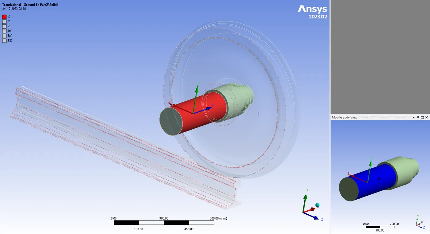 However, as can be seen from the model, the shaft will move in the X-Axis (shown in red), which is not parallel to the longitudinal axis of the Track.
Click the Shaft and Ground joint and choose Reference Coordinate System to align the shaft's X-Axis. Change the axis to Z in the Principal Axis section.
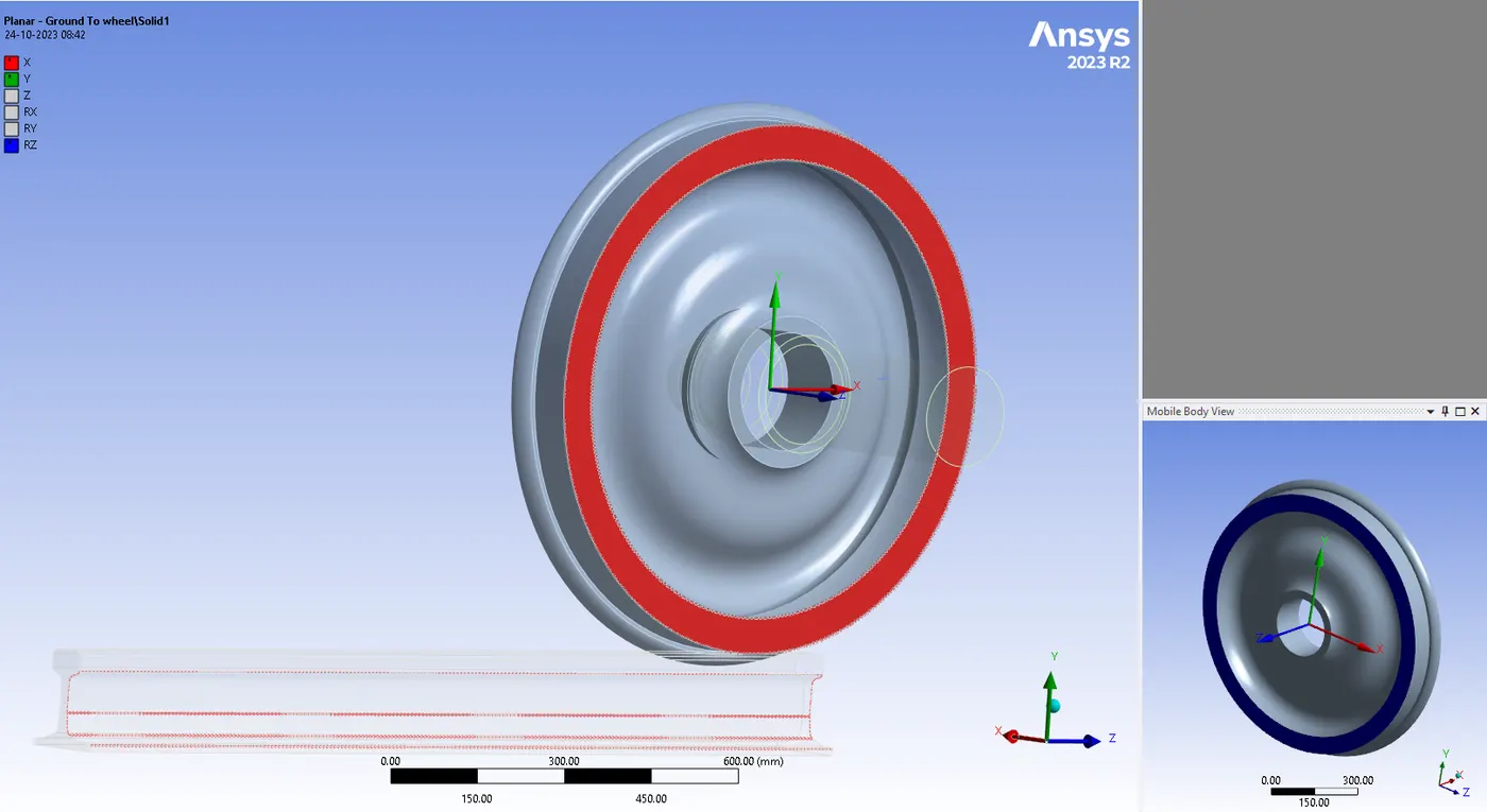
Now, add a planar joint in the geometry for the Wheel to remain in the current plane. To do so, add another joint, then select the Connection Type as Body-Ground and the Type as Planar Joint.
MESHING:
The 35 mm-sized elements used in the Railwheel Track assembly are mesh. To better capture structural behavior at the contact zone and speed up solution times, the element size on the regions of contact between wheel and track is likewise set at 15 mm using the face sizing option. There were 33309 nodes and 17975 elements altogether when all was said and done.
Face Sizing b/w track and wheel assy.
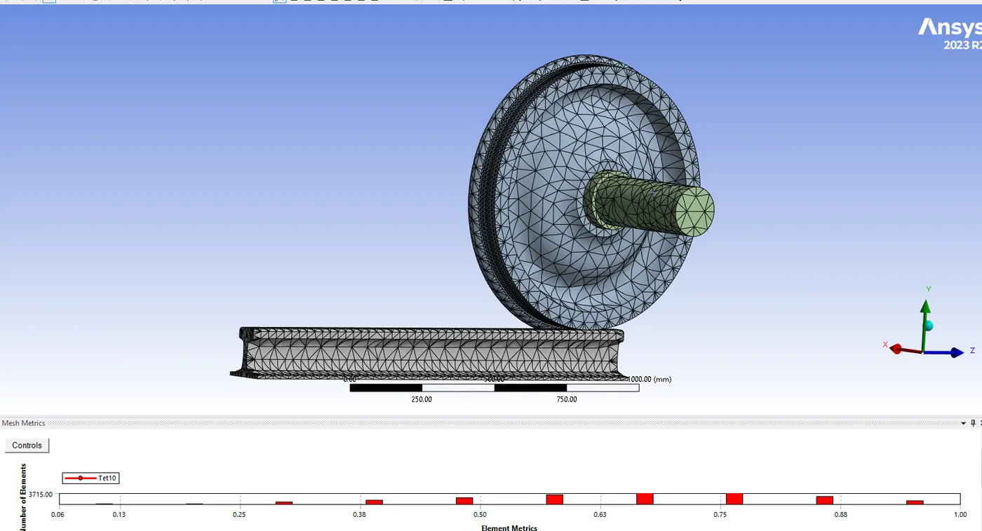
A mesh metric was used to identify elements based on their quality, and it can be observed that the elements of the lowest quality are minimal. Most elements have very high quality values ranging from 0.06 to 0.98 with an average value of 0.57. As a result, the mesh is of reasonable quality.
ANALYSIS SETTINGS:
The next step is to assign the Analysis Settings to the geometry. To do so, click on Analysis Settings and then:
- Set the Number of Steps equal to 5.
- Keep the Current Step Number as 1
- Auto Time Stepping as Program Controlled
- The Solver Type taken will be Direct.
Large Deflection is turned ON.
Force Convergence is turned ON.
Output Controls set the quantities to YES, as shown in the figure below:
Now for the remaining Time Steps, select all the remaining Time Steps
- Auto Time Stepping is turned ON
- Defined By is changed to Time, and
- Carry Over Time Step is turned ON.
- Minimum Time Step as 0.001 sec and
- Maximum Time Step as 0.1 sec.
The rest settings are the same as those done for the First Time Step.
- Two loads are applied after obtaining the analysis's setup parameters.
bearing load
displaced joint load
- 100000 N was applied as the bearing load between the wheel and shaft.
- Joint Displacement load:
- Joint: Translational – Ground to Shaft
- Type: Displacement
- Magnitude: Tabular Data
- Tabular Data is… from 0 to 500 mm
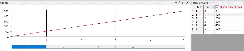
Next, select the inner surface of the Wheel and click on Loads, and select Bearing Load.
Magnitude is set to Components, and the load of magnitude 100 kN is applied on the surface in the negative Y-direction.
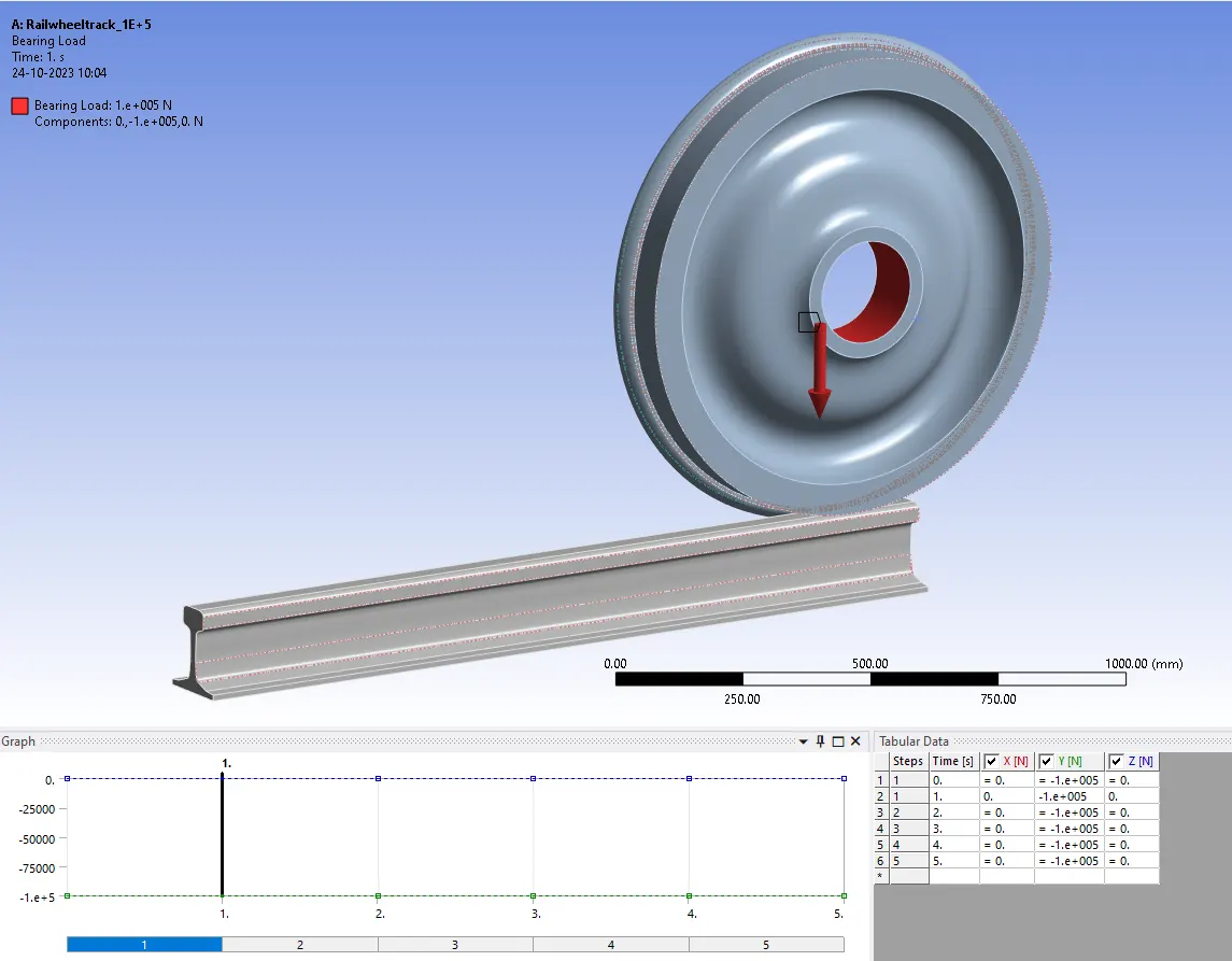
The same step for 500 KN has been repeated
POST-PROCESSING:
The derived results are for the running case as explained in the video for the bearing load of 100000N
1. TOTAL DEFORMATION
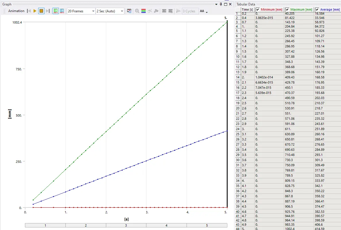
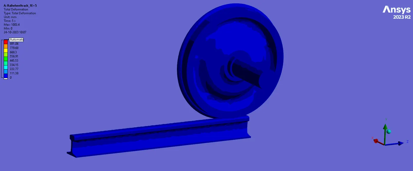
The total deformation of wheel and the track corresponding to the load acting on the body.
2. EQUIVALENT VON-MISES STRESS:
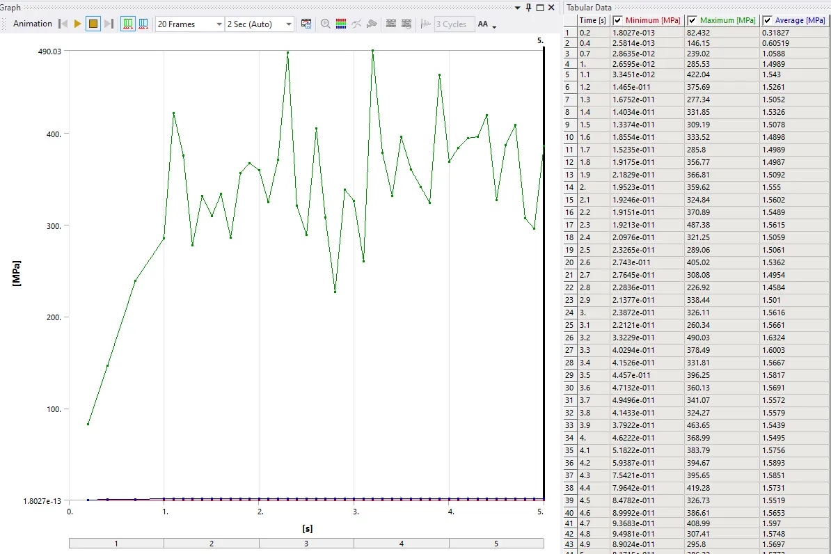
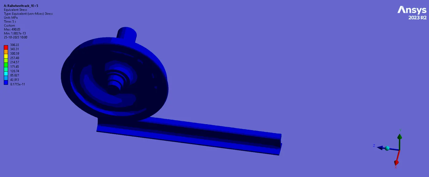
The stress developed at the respective load is 100000N is 386 Mpa
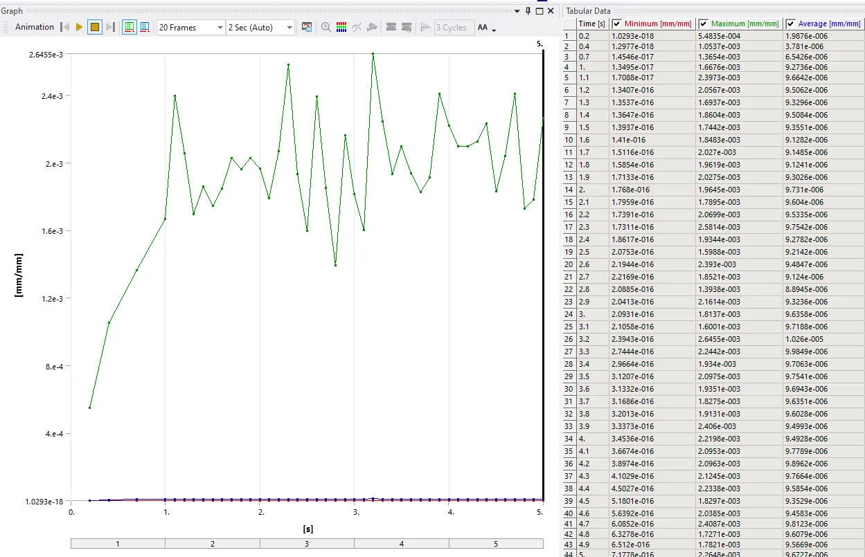
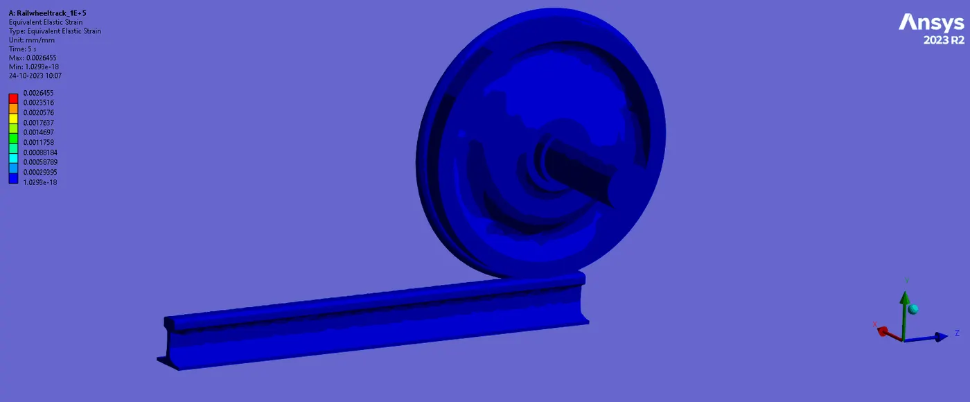
3. EQUIVALENT STRAIN:
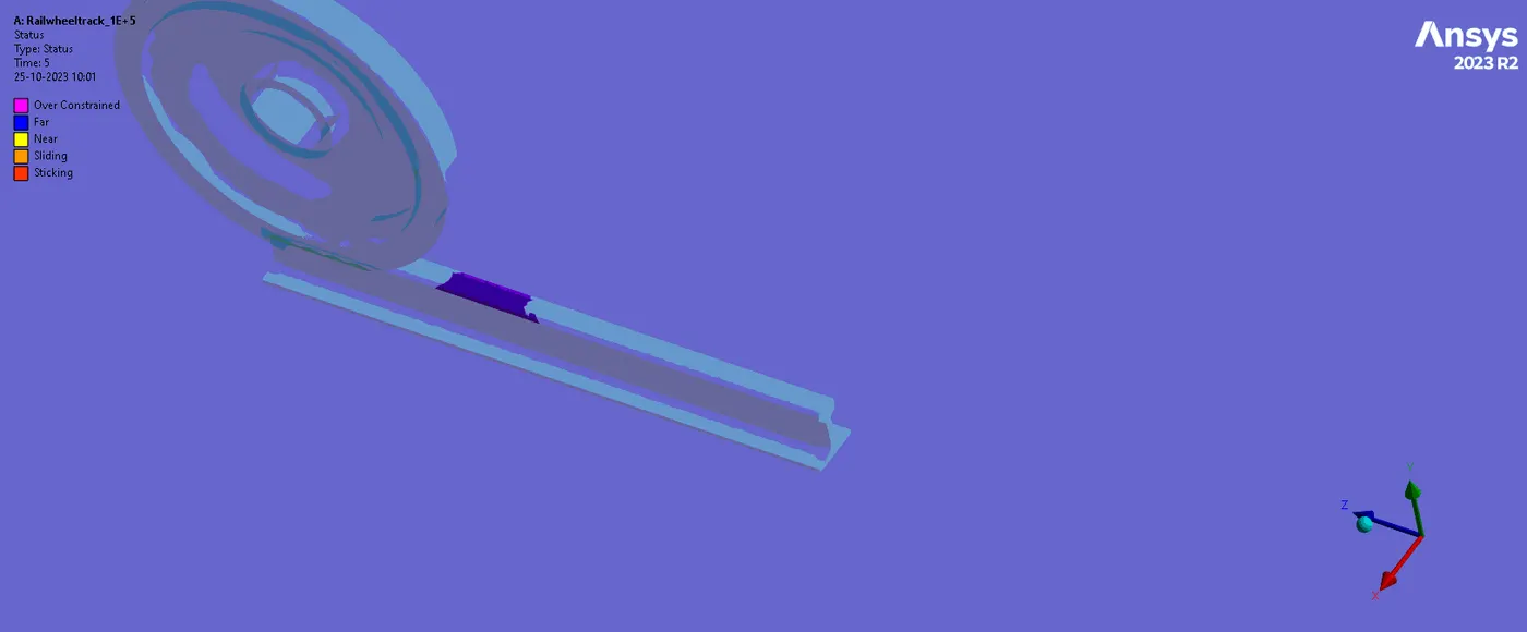
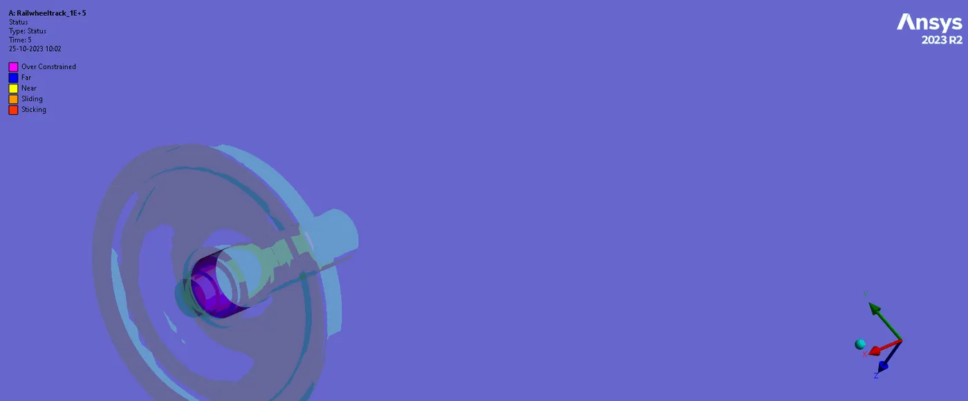
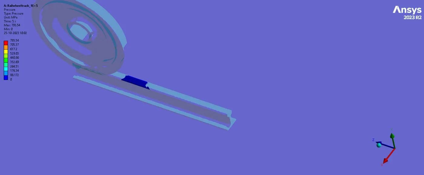
4. CONTACT STATUS:
5.FATIGUE TOOL LIFE:
CASE-2
The derived results are for the running case as explained in the video for the bearing load of 500000N
1. TOTAL DEFORMATION
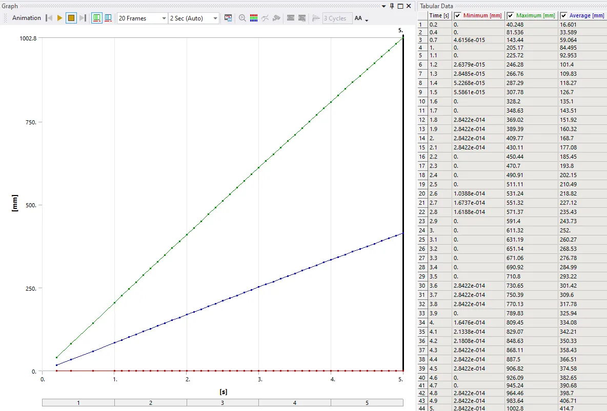
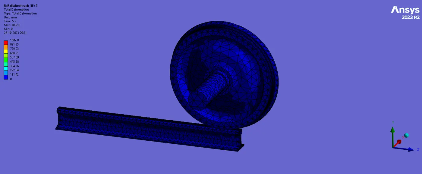
The total deformation of the wheel and the track correspond to the load acting on the body.
2. EQUIVALENT VON-MISES STRESS:
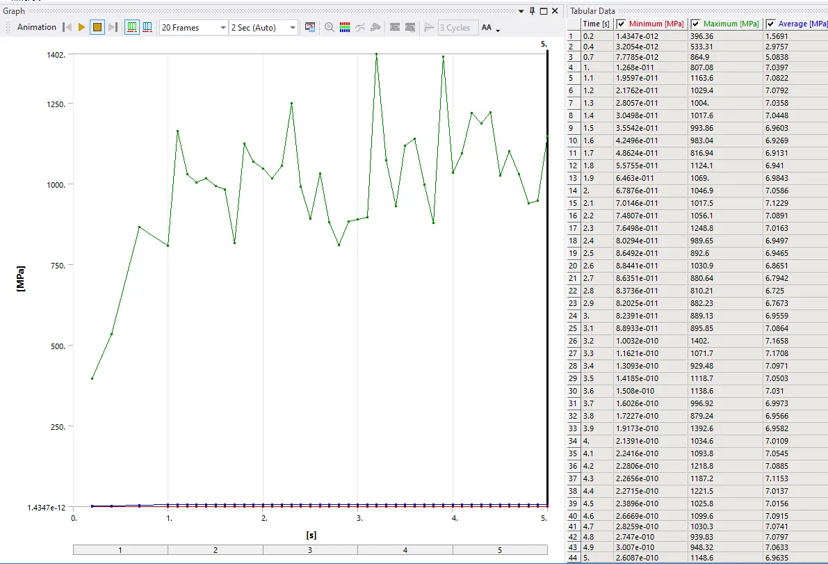
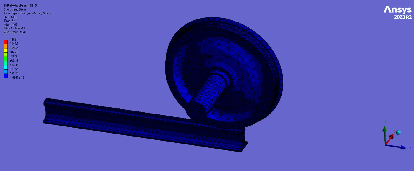
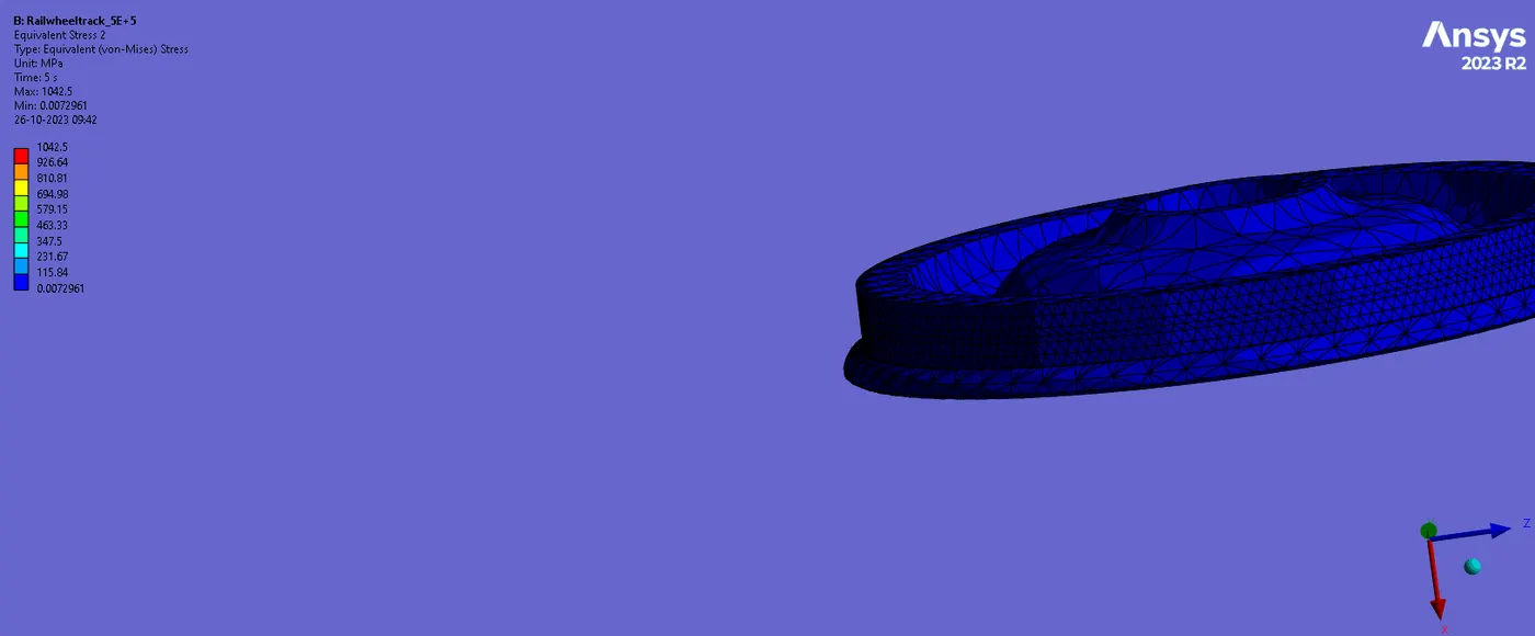
The stress developed at the respective load is 500000N is 1402 Mpa for the whole wheel and track but for the wheel only is 749 Mpa as shown below:
3. EQUIVALENT STRAIN:
4. CONTACT STATUS:
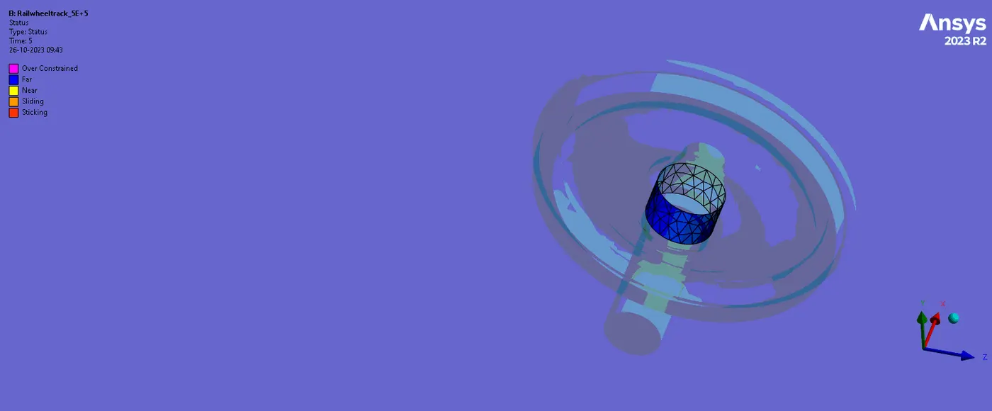
5.FATIGUE TOOL LIFE:
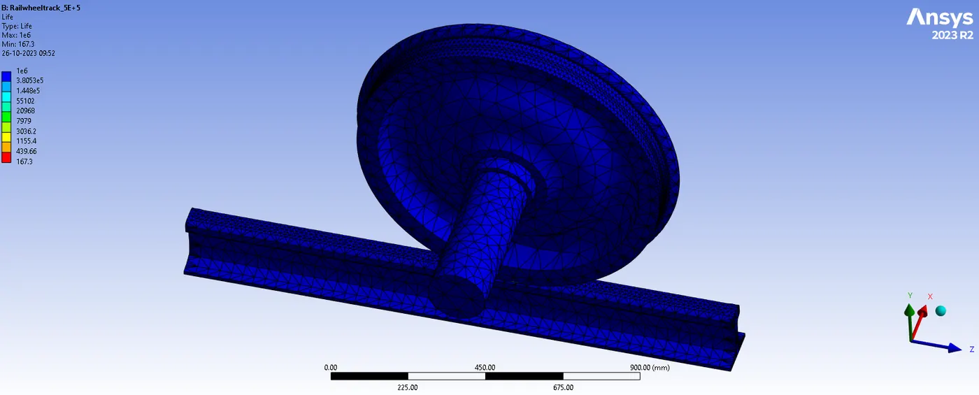
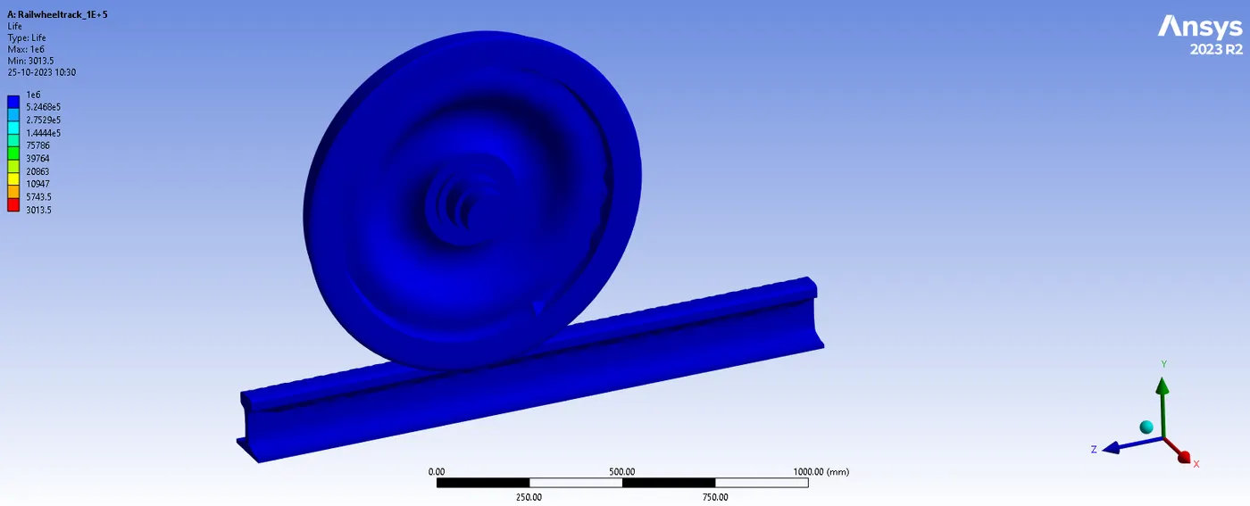
The result shows that the load increases, as the force on the trackwheel simulation the equivalent stress and deformation increases, the force is directly proportional to the stress value, and the life cycle for both loads is 1e^6 max.
COMPARISON:
| S No. | LOAD (N) | Maximum Deformation | Maximum Stress | Maximum Strain |
Fatigue Life (Max) |
Fatigue Life (Min) |
| CASE A | 100000N | 1002.4 mm | 386 MPa | 0.0026 mm/mm | 3013.5 | 1e+06 |
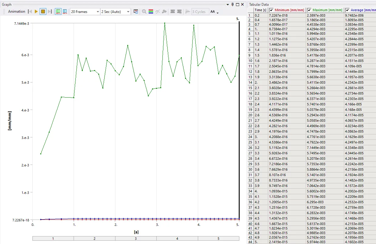
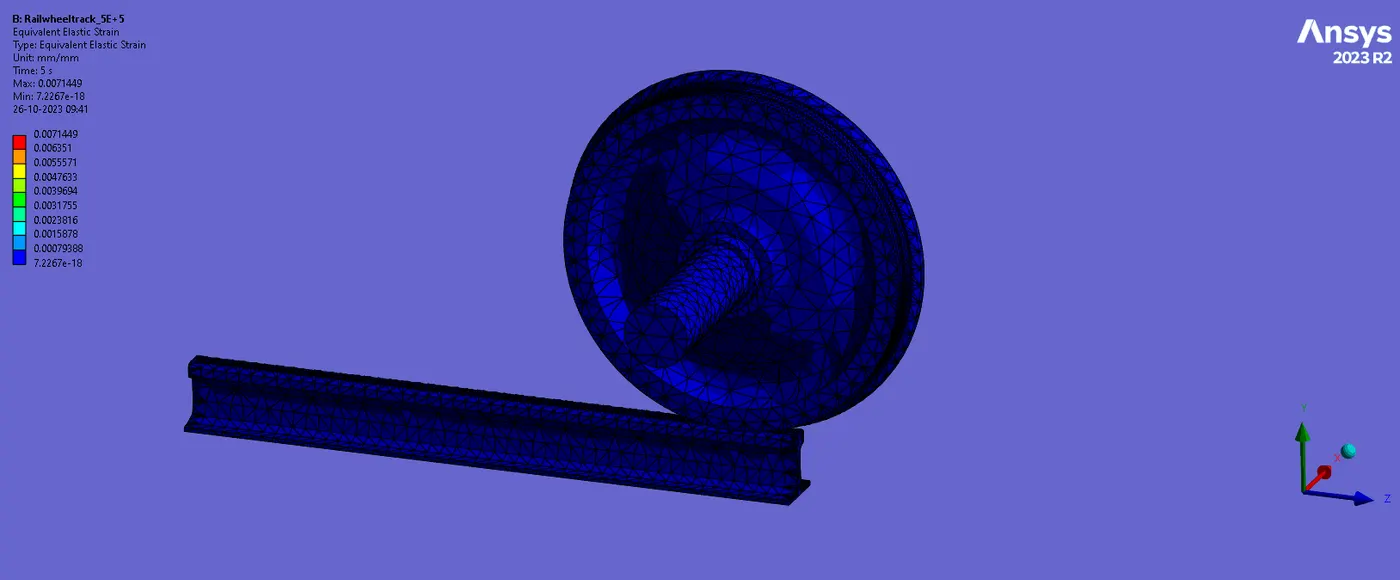
| CASE B | 500000N | 1002.8 mm | 1042 MPa | 0.0071 mm/mm | 167.3 | 1e+06 |
CONCLUSION
- According to the aforementioned study, the 50000 N bearing loading example has a shorter life cycle since it has greater comparable stress and equivalent elastic strain. For both scenarios, the overall distortion is determined to be comparable. In other words, the table shows that the value of total deformation is unaffected by an increase in the bearing load magnitude.
- When we compared the stress in the two scenarios, we discovered that when the load increased, the stress also increased in relation to the load. For example, the highest stress at 1E+5 N was 386 MPa, but it increased to 1042 MPa when the load was increased 3 times and the wheel's contact point is where the most stress is placed. Even though the rail can sustain a 50000 N bearing load case, the lifetime will be significantly shorter since the maximum value is greater than the yield stress value of the material.
- In this instance, the comparable strain value is likewise not affected by the load.
- When a component is loaded with a restricted load of 1E+5 N, its minimum fatigue life cycle is 3013.5 cycles, indicating that it has an infinite fatigue life. However, when a component is loaded with a 5-time load of 5E+5 N, its minimum fatigue life cycle is 1e+006 cycles, indicating that it has an infinite fatigue life. Hence the railway wheel track with the provided design dimension cannot be used for the 50000 N bearing load applications but can be used for the 10000 N case.
Case 3: Apply a user-defined result, compute the total deformation from it, and verify that it matches the result produced by ANSYS's built-in result for a load of 100,000 N.
Deformation data are frequently acquired as total deformation or directed deformation in ANSYS WorkBench. Both of these are used to calculate displacements based on stresses. The main difference is in the way the X, Y, and Z plane deformations are calculated by the directed deformation for a given system. In terms of total deformation, it gives the square root of the sum of the squares of the x, y, and z directions. The following formula yields a user-defined displacement result:
Total deformation is summision of each direction deformation , mathematically it can be expressed as
total deformation =square root of summision of square of each direction deformation
total deformation = sqrt(Ux^2+Uy^2+Uz^2)
Where,
Ux= deformation in x direction
Uy= Deformation in y direction
Uz= deformation in z direction
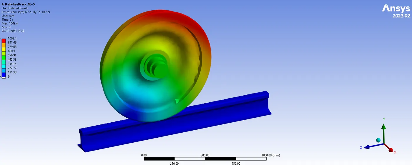
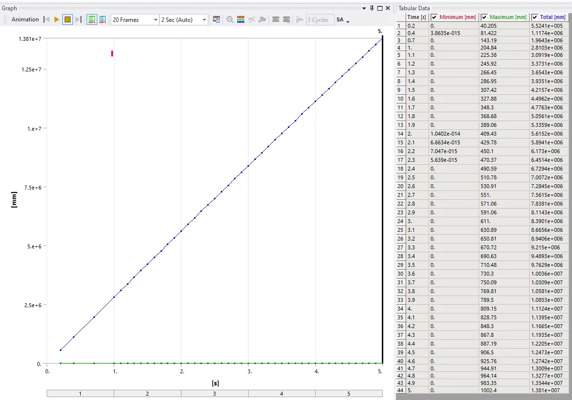
we check above equation in user define result in 1st case i.e. with load of 1E+5 N . we know that total deformation of inbuild system in ANSYS was 1002.4 mm
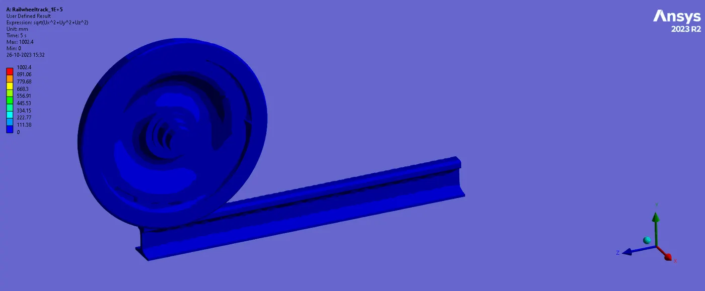
Total deformation has been found when using the expression in the user-defined area and that has become exactly the same as the one obtained from the original total deformation which is at the bearing load of 100000 N is 1002.4 mm.
The loading condition in CASE 2 is very severe and the wheel and track should not be put under such loading conditions.