Week 2 Railwheel and Track

Objective:

Perform a static structural analysis on the Railwheel and Track setup.

Rail wheel and track assembly is the most coomon component of a rail carriage. the load of the entire carriaage is borne by the shaft and wheel assembly and transferred on the the track through the wheel. It can be observed in the attached diagram below that the load of the carriage is transferred to the wheels eg. P1 & P2.

The shaft distributes the load of carriage evenly between the two wheels. This helps in maintaining a balance in the movement of the carriage.

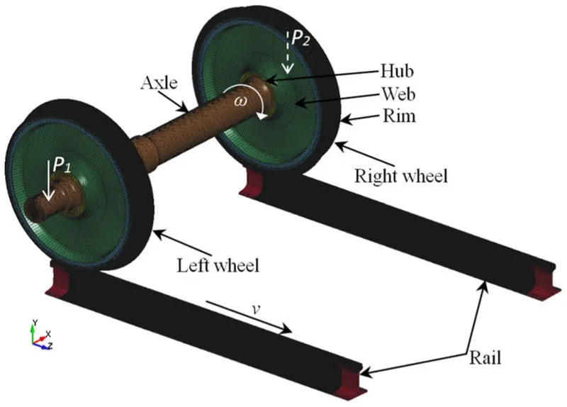
As per the problem statement, this analysis has been done in 2 parts, i.e. one with bearing load of `10^5 N` and one with a bearing load of `5 X 10^5 N`. Comparisons have been made for the two loads and results discussed.

Stages of  of simulation include:

Step 1: Geometry Creation

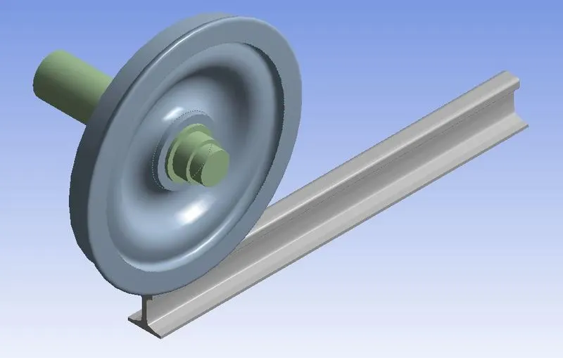
 The geometry was imported from the model of Railwheel and Track,

Step 2:  Material Selection

Default material selected was structural steel.

Properties for the material,

	Density	Young’s Modulus	Poisson’s ratio	Yield Strength	Ultimate Tensile Strength
Structural Steel	7850 Kg m^-3	200 GPa	0.3	250 MPa	460 MPa

Step 3: Meshing

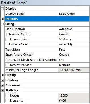
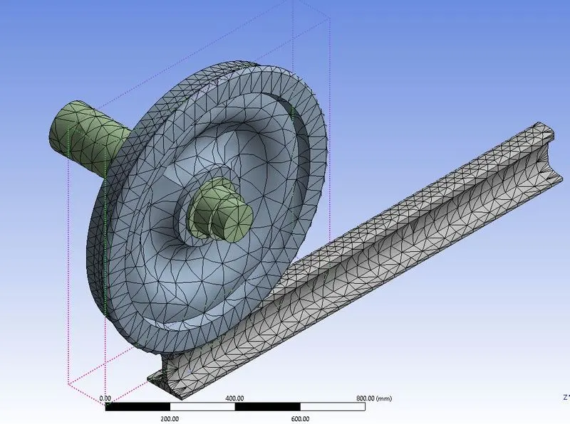
Meshing has been done based on following parameters,

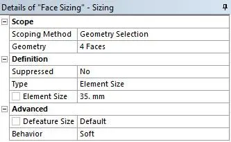
The parts in contact were meshed with a diferent element size of 35 mm for accurate results,

Step 4: Processing

Processing the model involves creation of connections, Joints, Bouindary conditions, Loads etc.

1. Creation of Connections:

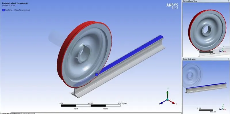
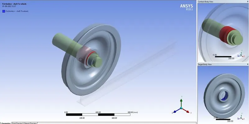
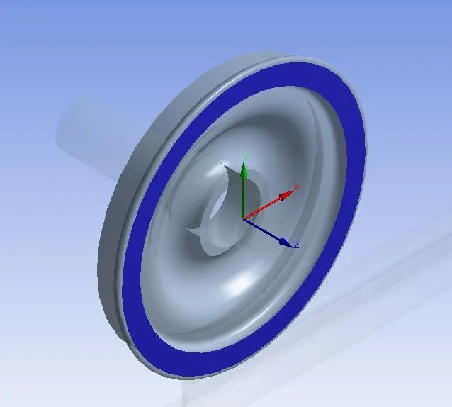
In the present problem, there are two sets of components in contact with each other i.e. shaft and wheel and wheel and track hence 2 conacts are established for thje same set.

• shaft and the wheel are in contact with each other at the hub. The connection between the shaft/axle  and the wheel is frictionless as the rotation is simultaeneous and no sliding takes place. hence, the contact between shaft and heel is taken as frictionless.
• Wheel and track connection is that of rolling friction. A friction coeffincient of 0.3 was taken to establish this contact.

 

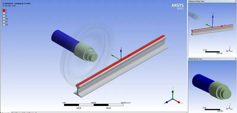
Three joint connections were created in order to define the model.

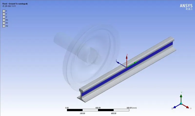
• First joint was created in the track/ rail to fix the rail in one position.
• A second connection was the joint on the wheel to fix it's plane of rotation.
• The final joint was made between shaft and the rail so as to establish translational relative motion between the two objects.

    

2. Analysis settings:

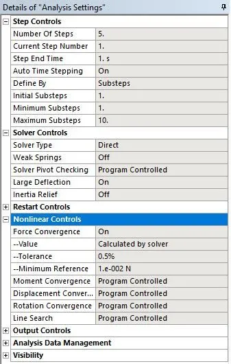
The no. of steps in this simulation was 5. The initial conditions were defined in step 1 and loading was done in consecutive steps to observe changes in the model more clearly.

In the first step, the auto timestepping feature is turned ON, and the substeps are defined by subset number ranging from 1-10. solver type is selected as 'direct' and large deflection option is switched ON. Forced convergence option in non-linear control is also switched ON.

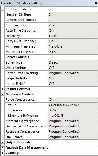
In the subsequent steps, auto timestepping feature is turned ON. Solver type is selected as 'direct' and large deflection option is switched ON. Forced convergence option in non-linear control is also switched ON.

The time step for iterations is set as,

• No. of steps- 4
• Auto time stepping- ON
• Defined by- time
• Initial time step- 0.1
• Minimum time step- 1E-3
• Maximum time step- 0.1

3. Application of loads:

To simulate the load of the carriage on the wheels, a bering load is applied on the circumference of inner radius of the wheel. A displacement of 100 mm/ time step is given to the shaft which in translation motion ot the rail.

Step 5: Results and Post-Processing

Case 1: Multiply the bearing load by 5 times and compare the results with the load of 100000 N (As done in week 2 video). Compare the Total Deformation, Equivalent stress, and the life under both the loads.

1. Total Deformation

   

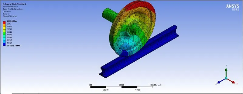
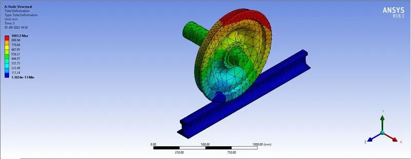
The total deformation in both cases has been shown here. The deformation is max at the top of the wheel since that end is the free end of the wheel and opposite to the point of application of resistance to the load.

   b. Equivalent stress

   

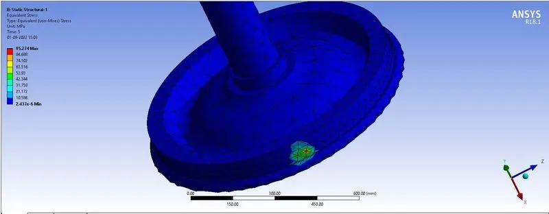
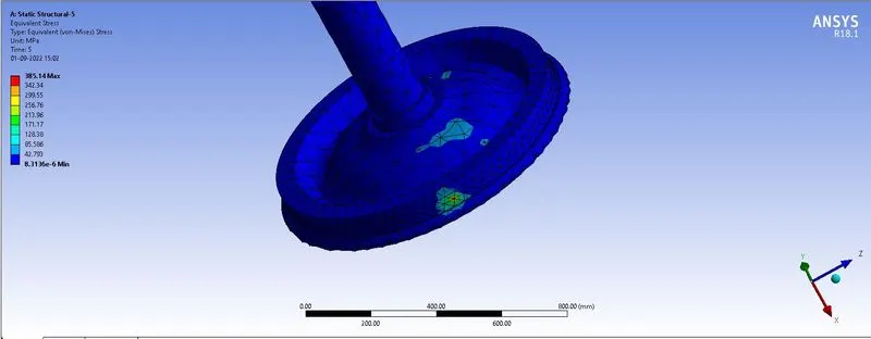
Equivalent stress on the bottom side side of the wheel is max since max laod is applied on the wheel and max resistance is faced by the bottom side of the wheel.

   c. Life of component

  

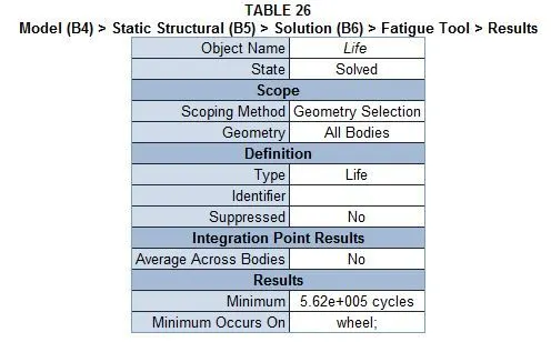
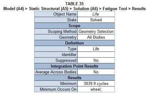
It is observed that under heavy loading, life of component is significantly reduced.

Case 2: Implement a User-defined result and calculate the Total Deformation from this result and check if it is the same as that obtained by the inbuilt result by ANSYS for a load of 100000 N.

While calculation user defined results, one needs to know the correct "expression" in order to implement required results. After a little research in the section of the software, the expression to find total deformation in the bodies was found. Afte implementing those instructions, the results are as follows,

   

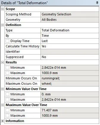
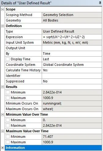
Max. deformation in results can be observed to be exactly the same in both cases.

Conclusions:

1. Case-1:

Results	Total Deformation (mm)	Equivalent Stress (MPa)	Fatigue life
Case-1	1000.9	95.274	5.62 * 10^5 cycles
Case-2	1001.2	385.14	3039 cycles

• Based on the analysis, is has been observed that the failure of this assembly occurs at the wheel.
• From above results, it can be observed that while the total deformation is similar in both cases of loading, the stresses on wheel are significantly higher in case of higher bearing load of 500000N.
• Due to this consistent high load, the life of the component is highly reduced. This is proven from the fact that the life wheel component under high loading is merely 3039 cycles as compared to 562000 cycles when loaded at 100000N.

Case-2:

Type	Max. Deformation	Min. Deformation
Total deformation	1000.9 mm	2.8422*10^-14 mm
User defined	1000.9 mm	2.8422*10^-14 mm

• It is evident that the maximum and minimum deformation completely matches in either case of user defined or system generated deformation values.