Week 4.1 - Genetic Algorithm

What are Genetic Algorithms?

Genetic algorithms are a part of a bigger group of algorithms called evolutionary algorithms and are a learning method inspired by evolutionary biology. 

The process of natural selection starts with the selection of the fittest individuals from a population. They produce offspring which inherit the characteristics of the parents and will be added to the next generation. If parents have better fitness, their offspring will be better than parents and have a better chance at surviving. This process keeps on iterating and in the end, a generation with the fittest individuals will be found.

This notion can be applied for a search problem. We consider a set of solutions for a problem and select the set of best ones out of them.

Five phases are considered in a genetic algorithm.

1. Initial population
2. Fitness function
3. Selection
4. Crossover
5. Mutation

Initial Population

• Every gene represents a parameter (variables) in the solution. This collection of parameters that forms the solution is the chromosome. Therefore, the population is a collection of chromosomes. 
• Order of genes on the chromosome matters.
• Chromosomes are often depicted in binary as 0’s and 1’s, but other encodings are also possible.

Fitness Function

• We have to select the best ones to reproduce offspring out of the available chromosomes, so each chromosome is given a fitness value.
• The fitness score helps to select the individuals who will be used for reproduction.

Selection

• This phase’s main goal is to find the region where getting the best solution is more.
• Inspiration for this is from the survival of the fittest.
• It should be a balance between exploration and exploitation of search space.
• GA tries to move the genotype to higher fitness in the search space.
• Too strong fitness selection bias can lead to sub-optimal solutions.
• Too little fitness bias selection results in an unfocused search.
• Thus, Fitness proportionate selection is used, also known as roulette wheel selection, as a genetic operator used in genetic algorithms to select potentially useful recombination solutions.

Generation of offsprings happen in 2 ways:

1. Crossover
2. Mutation

Crossover

Crossover is the most vital stage in the genetic algorithm. During crossover, a random point is selected while mating a pair of parents to generate offsprings.

There are 3 major types of crossover.

•  Single Point Crossover: A point on both parents’ chromosomes is picked randomly and designated a ‘crossover point’. Bits to the right of that point are exchanged between the two parent chromosomes.
• Two-Point Crossover: Two crossover points are picked randomly from the parent chromosomes. The bits in between the two points are swapped between the parent organisms.
• Uniform Crossover: In a uniform crossover, typically, each bit is chosen from either parent with equal probability.

The new offspring are added to the population.

 Mutation

In a few new offspring formed, some of their genes can be subjected to a low random probability mutation. This indicates that some of the bits in the bit chromosome can be flipped. Mutation happens to take care of diversity among the population and stop premature convergence.

Convergence:- When there is no improvement in the solution quality after completing a certain number of generations set beforehand, the algorithm stops. Or When a hard and fast range of generations and time is reached or if a limit is set to the function till an acceptable solution is obtained.

SYNTAX:-

Based on the type of program(inputs, variables, output required), the syntax for GA can be chosen from a host of syntaxes,

1. x = ga(fun,nvars) finds a local unconstrained minimum, x, to the objective function, fun. nvars is the dimension (number of design variables) of fun.
2. x = ga(fun,nvars,A,b) finds a local minimum x to fun, subject to the linear inequalities A*x ≤ b. ga evaluates the matrix product A*x as if x is transposed (A*x').
3. x = ga(fun,nvars,A,b,Aeq,beq) finds a local minimum x to fun, subject to the linear equalities Aeq*x = beq and A*x ≤ b. (Set A=[] and b=[] if no linear inequalities exist.) ga evaluates the matrix product Aeq*x as if x is transposed (Aeq*x').
4. x = ga(fun,nvars,A,b,Aeq,beq,lb,ub) defines a set of lower and upper bounds on the design variables, x, so that a solution is found in the range lb ≤ x ≤ ub. (Set Aeq=[] and beq=[] if no linear equalities exist.)
5. x = ga(fun,nvars,A,b,Aeq,beq,lb,ub,nonlcon) subjects the minimization to the constraints defined in nonlcon. The function nonlcon accepts x and returns vectors C and Ceq, representing the nonlinear inequalities and equalities respectively. ga minimizes the fun such that C(x) ≤ 0 and Ceq(x) = 0. (Set lb=[] and ub=[] if no bounds exist.)
6. x = ga(fun,nvars,A,b,Aeq,beq,lb,ub,nonlcon,options) minimizes with the default optimization parameters replaced by values in options. (Set nonlcon=[] if no nonlinear constraints exist.) Create options using optimoptions.
7. x = ga(fun,nvars,A,b,Aeq,beq,lb,ub,nonlcon,intcon) or x = ga(fun,nvars,A,b,Aeq,beq,lb,ub,nonlcon,intcon,options) requires that the variables listed in intcon take integer values.
8. x = ga(problem) finds the minimum for problem, a structure described in problem.
9. [x,fval] = ga(___), for any previous input arguments, also returns fval, the value of the fitness function at x.
10. [x,fval,exitflag,output] = ga(___) also returns exitflag, an integer identifying the reason the algorithm terminated, and output, a structure that contains output from each generation and other information about the performance of the algorithm.
11. [x,fval,exitflag,output,population,scores] = ga(___) also returns a matrix population, whose rows are the final population, and a vector scores, the scores of the final population.

STALAGMITE FUNCTION:

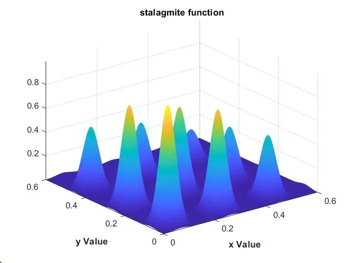
The following equations are used in the stalagmite function to plot the graph in the main functions,

`f(x,y) = f_(1,x)*f_(2,x)*f_(1,y)*f_(1,y)`-------------------------(1)

`f_(1,x) = [sin(5.1*pi*x+0.5)]^6`---------------------------------(2)

`f_(2,x) = exp(-4*log(2)*(x-0.0667)^2/0.64)`-------------------(3)

`f_(1,y) = [sin(5.1*pi*y+0.5)]^6`---------------------------------(4)

`f_(2,y) = exp(-4*log(2)*(y-0.0667)^2/0.64)`-------------------(5)

A stalagmite function is created to be called in the main function to be maximized. 

%fitness function to be maximized
function [f] = stalagmite(ip_vector)
%inputs to the function
x = ip_vector(1);
y = ip_vector(2);

%%standard formulation of stlalagmite fuinction
f1_x = (sin(5.1*pi*x + 0.5))^6;
f1_y = (sin(5.1*pi*y + 0.5))^6;
t1 = ((x-0.0667)^2)/(0.64);
f2_x = exp(-4.*log(2)*t1);
t2 = ((y-0.0667)^2)/(0.64);
f2_y = exp(-4.*log(2)*t2);

%%negative value of f so that maixmization and not minimization of function
%occurs
f = -(f1_x.*f2_x.*f1_y.*f2_y);
end

 While using the function at the end as we are using the -ve sign so that the plot will be reversed as we have to find the maxima of the given function using ga.

CODE TO PLOT STLAGMITE FUCNTION:

clear
close all
clc
%% PROVIDING THE SEARCH SPACE FOR THE FUNCTION
x=linspace(0,0.6,150);
y=linspace(0,0.6,150);
[xx,yy]=meshgrid(x,y);
num_cases=50; %Number of itreation for which the function will evaluate the fitness
%% CREATING THE SURFACE PLOT OF STALAGEMITE FUNCTION
for i=1:length(xx)
for j=1:length(yy)
input_vector(1)=xx(i,j);
input_vector(2)=yy(i,j);
f(i,j)=stalagmite(input_vector); %values of function in given search space
end
end
surfc(xx,yy,-f); %generating the surface
title ('stalagmite function','BackgroundColor','w');
xlabel ('x Value','FontWeight','bold','BackgroundColor','w');
ylabel('y Value','FontWeight','bold','BackgroundColor','w');

%To SMOOTHEN THE CURVE
shading interp 

ALGORITHM:

• Create the mesh from the two vectors which will be acting as a search space to find the maxima of the function.
• Create the mesh of these two vectors using the ‘mesh’ command and define the no. of iterations as num_cases to iterate the values of the optimum values of the function.
• calculate the values of fitness function at each point of the mesh grid formed.
• Create its surface through ‘surfc’ command which will also provide the contour of the generated surface.
• While using surfc applying the -ve sign to the function will generate the surface upside down which will be quite good to get the maxima of the function, as it will provide a positive value for the maxima using the -ve sign.

OUTPUT:

CODE TOP MAXIMIZE STALAGMITE FUNCTION:

clear
close all
clc
%% PROVIDING THE SEARCH SPACE FOR THE FUNCTION
x=linspace(0,0.6,150);
y=linspace(0,0.6,150);
[xx,yy]=meshgrid(x,y);
num_cases=50; %Number of itreation for which the function will evaluate the fitness
%% CREATING THE SURFACE PLOT OF STALAGEMITE FUNCTION
for i=1:length(xx)
for j=1:length(yy)
input_vector(1)=xx(i,j);
input_vector(2)=yy(i,j);
f(i,j)=stalagmite(input_vector); %values of function in given search space
end
end
surfc(xx,yy,-f); %generating the surface
title ('stalagmite function','BackgroundColor','w');
xlabel ('x Value','FontWeight','bold','BackgroundColor','w');
ylabel('y Value','FontWeight','bold','BackgroundColor','w');

shading interp %To remove the lines produced by the mesh grid

% STATISTICAL BEHAVIOUR (UNBOUNDED)
tic %calculating the study time through tic and toc command
for i=1:num_cases
[inputs,fop(i)]=ga(@stalagmite,2); %calculating the optimized value of the function
xop(i)=inputs(1); %at each iteration
yop(i)=inputs(2);
end
study1_time=toc %displaying the time taken to evaluate
% PLOTING THE GRAPH
figure(1)
subplot(2,1,1)
surfc(xx,yy,-f);
hold on
shading interp
plot3(xop,yop,-fop,'marker','o','markersize',5,'markerfacecolor','r');
xlabel('x Value','BackgroundColor','w', 'FontWeight','bold');
title ('Unbounded inputs', 'BackgroundColor','w');
ylabel('y Value', 'BackgroundColor','w', 'FontWeight','bold');
grid on
subplot(2,1,2)
plot(-fop);         
xlabel('iterations','BackgroundColor','w', 'FontWeight','bold');
ylabel('function min value','BackgroundColor','w', 'FontWeight','bold');

%% STATISTICAL BEHAVIOUR (BOUNDED)
tic %calculating the study time through tic and toc command
for j=1:num_cases

%calculating the optimized value of the function
[inputs,fop(j)]=ga(@stalagmite,2,[],[],[],[],[0;0],[1;1]); 
%at each iteration with boundation
xop(j)=inputs(1); 
yop(j)=inputs(2);
end
study2_time=toc

%PLOTTING
figure(2)
subplot(2,1,1)
hold on
surfc(xx,yy,-f)
shading interp
plot3(xop,yop,-fop,'marker','o','markersize',5,'markerfacecolor','r');
title ('Bounded inputs', 'BackgroundColor','w');
xlabel('x Value','BackgroundColor','w', 'FontWeight','bold');
ylabel('y Value', 'BackgroundColor','w', 'FontWeight','bold');
grid on
subplot(2,1,2)
plot(-fop);
xlabel('iterations','BackgroundColor','w', 'FontWeight','bold');
ylabel('function min value','BackgroundColor','w', 'FontWeight','bold');

%% MODIFYING THE NUMBER OF POPULATION
%increaing the size of population by using optimoptions function
options=optimoptions('ga','populationsize',300) 
tic
for k=1:num_cases
[inputs,fop(k)]=ga(@stalagmite,2,[],[],[],[],[0;0],[1;1],[],[],options);
xop(k)=inputs(1);
yop(k)=inputs(2);
end
study3_time=toc

%PLOTTING
figure(3)
subplot(2,1,1)
hold on
surfc(xx,yy,-f)
shading interp
plot3(xop,yop,-fop,'marker','o','markersize',5,'markerfacecolor','r');
title ('Bounded inputs with updated population size', 'BackgroundColor','w');
xlabel('x Value','BackgroundColor','w', 'FontWeight','bold');
ylabel('y Value','BackgroundColor','w', 'FontWeight','bold');
grid on
subplot(2,1,2)
plot(-fop);
xlabel('iterations','BackgroundColor','w', 'FontWeight','bold');
ylabel('function min value','BackgroundColor','w', 'FontWeight','bold');

STATISTICAL STUDY WITHOUT BOUNDATION (Study-1)

In this step, the optimum value of the fitness function at each iteration is calculated using the above-mentioned syntax. Then it is plotted into the 'surf' command, providing the optimum values of the function and its variation. Also, tic and tok command is used to evaluate the time used for optimizing the function.

From the results, it is clear from 'ga study-1', that the results are not quite accurate and include a lot of variation in optimizing the function.

STATISTICAL STUDY WITH BOUNDATION (Study-2)

The difference between study with foundation and previous study is in providing the upper and the lower limit in the ga so that the search space is reduced with the upper and lower boundary. Plotting is similar to the above study-1.

It is clearly seen from the 'ga study-2', that after providing the boundary limits the variation in the optimum value of the function has reduced.

STATISTICAL STUDY WITH INCREASE IN SIZE OF POPULATION (Study-3)

This study uses the ‘optimoptions’ command to increase the size of the population. The benefit is that it works on a large set of numbers which will be lead to an increase in the possibility of finding the better fitness of the function.

The drawback is that the time for evaluation will increase.

ALGORITHM FOR OPTIMIZATION CODE:

• Clearing workspace, command window & closing all plots.
• Define our search space by using linspace command.
• Calculating a 2D  mesh using meshgrid command.
• Evaluating the stalagmite function for each value of x & y.
• using ga command with unbounded inputs means optimum value may be come from outside of search space.
• ga command with bounded inputs gives an optimum value from inside of search space. However, there is a large variation in optimum value. 
• GA command with bounded inputs gives an optimum value from inside of search space. However, this time to avoid huge variation in optimum value, initial population size has been increased to 300. If initial population is not specified in the program, MATLAB assumes 50 as initial population.

RESULTS:

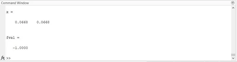
The stalagmite function has a maximum value of 1 at given x and y coordinates. since the function was defined with a negative value, the value returned was also in the negative. 

ERRORS:

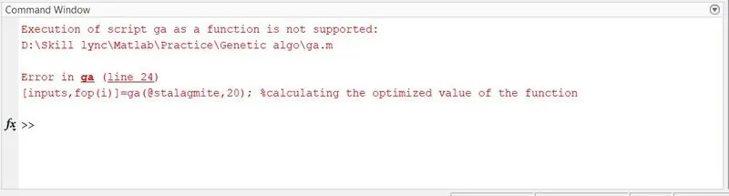
1. Execution of script roots as a function is not supported

Error Resolution:

Initially, the program file was stored in the directory as 'ga' which is a default function in matlab. So, when the file was named as 'ga', the software associated the term ga with the program file and not the function. So when the genetic algorithm function was called in line 24, it read the command with ga as a script and not a function.

Upon researching about the error, the file name was changed and the function ran smoothly.

References:-

1. https://in.mathworks.com/help/gads/what-is-the-genetic-algorithm.html
2. https://in.mathworks.com/help/gads/how-the-genetic-algorithm-works.html
3. https://skill-lync.com/knowledgebase/genetic-algorithm-explained
4. https://in.mathworks.com/help/gads/ga.html?s_tid=doc_ta#mw_f69991d0-5b23-4023-8c8e-e2890f2474d5