Week 3 - Solving second order ODEs

A simple pendulum consists of a ball (point-mass) m hanging from a (massless) string of length L and fixed at a pivot point P. When displaced to an initial angle and released, the pendulum will swing back and forth with the periodic motion.

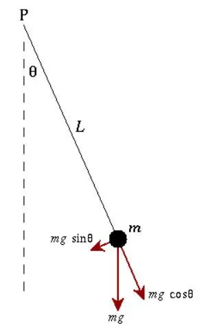
By applying Newton's second law for rotational systems, the equation of motion for the pendulum may be obtained,

`(d^2θ)/ dt^2 + g L sin θ = 0`

In the case of a damper with damping co-efficient 'b', the equation changes to,

`(d^2θ)/ dt^2 + b/m*((dθ)/dt) + g L sin θ = 0`----------------------------------------- (1)

in order to convert this 2nd order ODE to a 1st order ODE, let us make some assumptions,

`theta = theta_1`,

therefore, `(d theta)/dt = (d theta_1)/dt`

Also, let

`(d theta)/dt = theta_2`----------------------------------(2)

therefore, `(d^2θ)/ dt^2= (d theta_2)/dt`----------------(3)

So now we have equation 2 & 3 instead of only equation 1 to solve the ODE.

solution matrix for `theta` can be written as,

`d/dt[(theta_1), (theta_2)] = [[theta_2], [-b/m*(theta_2)-g/l*sin(theta_1)]]`

To solve this system of 1st order ODE's, matlab has a function 'ode45'.

• Algorithm for the program

1. Creating solution matrix `theta`:

In order to solve the `2^(nd)`order ODE, it is converted into a system of 1st order ODE's. This system of ODE's was defined in a separate function to be called in the main program to be solved by ode45. This is done in the same method as demonstrated in the derivation above. The function was named 'ode_sol'.

2. Code to solve ODE:

ode45 is a function in Matlab that solves ODE's and PDE's using `4^(th)`order Runge Kutta method. The inputs required are the function of the system of our ODE's, the initial conditions and lastly the time interval across which the function has to be integrated. In the function defined, the inputs other than variables are length of arm (l), mass of bob (m), acceleration due to gravity (g) and damping coefficient (b). after defining the required inputs, the ode45 function integrates our defined function 'ode_sol' across defined time interval. The solution can then be plotted in terms of angular displacement (`theta`) and angular velocity `(d theta)/dt`.

1. clear all - Removes items from workspace, freeing up system memory.

   close all - Closes all figures except those listed by the user.

   clc - clears all data from the command window.

2. All inputs to the function as well the code are listed viz., length of arm (l), mass of bob (m), acceleration due to gravity (g) and damping coefficient (b).
3. Initial conditions and limit of integration are defined with column vector 'theta' and row vector 't' respectively.
4. Array [t, result] stores the results from the solution of 'ode_sol' by ode45. The first column of the vector contains angular displacements of the pendulum at all angles in the given time limit. The second column of the vector contains the angular velocity of the bob of the pendulum for the corresponding displacement.
5. Both displacement and velocity are plotted on the same graph.
6. To animate the motion of the pendulum, the position of the bob of the pendulum has to be known at every point. Based on values of angular displacement, the position of the bob can be found out as x1 and y1. A for loop calculates all values of x1 & y1 for the entire range of `theta` and plots it in figure 2.
7. The fixed point of the pendulum is plotted at (0,0).
8. All frames of the plot in figure 2 are captured in file V by the 'getframe' command and the loop is reset for the next value of `theta`.
9. The file V is then converted into a .avi file (video).

3. Code:

1. Function to define solution matrix theta:

function [dtheta_dt] = ode_sol(t, theta, l, m, g, b)

theta1 = theta(1);
theta2 = theta(2);

dtheta1_dt=theta(2);
dtheta2_dt=-b/m*theta2 - g/l*sind(theta1);

dtheta_dt = [dtheta1_dt;dtheta2_dt];
end

ii. Code to solve ODE:

clear all
close all
clc

%length of the pendulum, l(m)
l= 1;

%mass attached to the pendulum, m(kg)
m= 1;

%Acceleration du to gravity in m/s2,
g = 9.81;

%damping coefficient, b
b=0.05;

%initial conditions,
%angular displacement = 0
%velocity 3 rad/s
theta= [0;3];

%limit of integration
t = linspace(1,20);

%calling ode_sol function to solve the ODE with ode45 solver
%t and theta are the variables to the function and are defined as such with
%@(t, theta)
%l, m, g, b are all constants who's values are also inputs to the function
%The t in the function after the function is declared gives the limits to
%the integration of theta variable. the theta input, in the end, gives the
%initial conditions on the problem and is declared in line 20 of this code
[t, results] = ode45(@(t, theta) ode_sol(t, theta,l,m,g,b),t, theta);

figure (1)

%plots displacement who's value is in the first row of the results matrix
plot(t,results(:,1),'LineWidth',2);
hold on

%plots velocity who's value is in the first row of the results matrix
plot(t,results(:,2),'LineWidth',2);

%xlabel & ylabel commands labels x & Y axis respectively and legend creates 
% a legend of the curve 
ylabel('Plot');
xlabel('Time');
legend ('Displacement', 'Velocity');
grid on

%To create the animation of a pendulum, values of angular disp. is stored in an array 'x' 
[x] = results(:,1);

%the for loop calculates the position of the pendulum for each value of angular
%displacement and plots it in figure 2. the procedure repeats for all
%values of angular displacement and all the frames(plots) are saved in V(i) to
%create and animation
for i = 1:length(x)
theta3 = x(i);

%coordinates of the fixed end of the pendulum
xo=0;
yo=0;

%coordinates of pendulum bob
x1=l*sind(theta3);
y1=-l*cosd(theta3);
figure (2)
plot([xo x1], [yo y1], "Color",'k', 'Marker','o', 'MarkerSize',15,'MarkerFaceColor','m');
axis([-0.12 0.12 -1 0])
pause(0.25)

%To capture each plot of x1, y1 as a frame to compile into animation
V(i)=getframe(gcf);
end
%resets the for loop to the higher value of i 
i=i+1;

%creates and stores avi type of animation file
movie(V);
animationfile=VideoWriter('ODE_sol', 'Uncompressed AVI');
open(animationfile);
writeVideo(animationfile,V);
close(animationfile);

4. Errors faced while the development of code

1. Kindly refer to the video file '2R_robotic_arm-error2' in the link below to find the error in the animation,

https://drive.google.com/drive/folders/1YdqlfNyTw8agEXDARjWjLCX42jt6iYKk?usp=sharing

It can be observed that the animation was not stable and values of the axes were changing haphazardly. The reasoning observed was that the axes limiting command was not included in the code. hence the 'axis' command was included to limit the value of x axis in the plot.

Error resolution: The 'axis' command was included in the code so that it gets assimilated in the plot.

ii.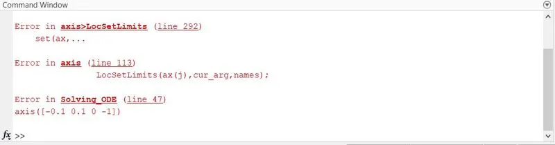

Error in syntax was observed as a smaller value of limit was written on the right side

Error resolution: The syntax was corrected and values of the axes were updated as per the output of displacement from the first half of the code