Week 2 - Flow over a Cylinder.

Objective :- To simulate the flow over a cylinder with the steady and unsteady case & study of effects of Reynolds no. and Karman vortex phenomenon.

Introduction :-

Vertex shedding - When the boundary layer seperates they create a shear layer and they are inherently unstable because they have inflation points in their velocity profiles,They develop waves that then rollup into vortices.There are two approxly parallel shear layers behind a bluff-body like cylinder,On outside(top) the flow goes forward & inside it goes backwards.Then the shear layers start interacting by snaking up & down together.soon they will rollup into vertices that are shed alternatively from each side of cylinder causing of vertex shedding.

Von Karman vortex street - The fluid stream fails to stick to the shape of the bluff body over which it flows, but breaks off behind it resulting in what is known as the wake region. And it is this wake that constitutes the stage for the dramatic fluid dynamic phenomenon known as the Karman vortex street.

In the wake of the cylinder, the flow pattern consists of an alternating system of vortices or regions of rotation. A clockwise rotating eddy or vortex is 'shed' from the top side, followed by an anticlockwise rotating vortex from the bottom side, and this process continues leading to a staggered system of alternating vortices.

History :

In 1911, the celebrated German fluid dynamicist Ludwig Prandtl was investigating the static pressure distribution along the surface of a circular cylinder when it was placed in a steady stream of water. Karman, who at the time was a graduate assistant working with PrandtlKarman showed that the observed vortex system of staggered asymmetrical vortices was the only stable system. And it is only a stable configuration that one gets to observe in practice. And it is only a stable configuration that one gets to observe in practice. This contribution, which was presented to the Gottingen Academy by Prandtl and a subsequent paper, are in fact Karman's contribution to this phenomenon. Over time, this contribution of Karman resulted in the pattern being called the Karman Vortex Street.

Part 1 - Simulation of the steady and unsteady case and calculating the Strouhal Number for Re= 100.

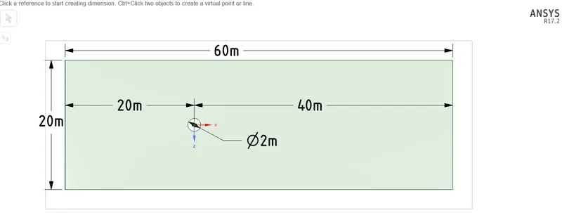
Goemetry Creation :

• 2D Simulation is proccessed in a rectangular space.
• All dimensions are in Meters.

Mesh creation:

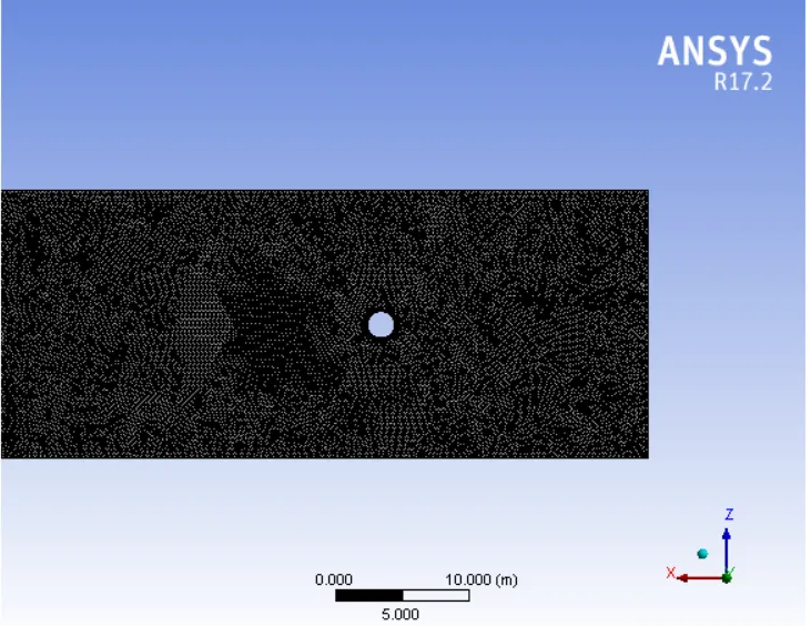
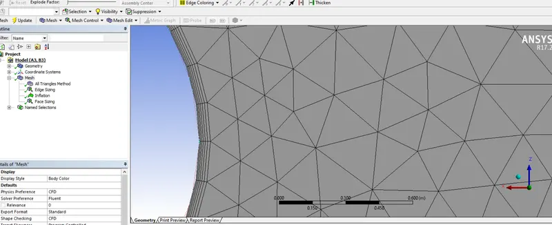
• All the mesh element structure was changed to traingles method with fine mesh size of 0.25m.
• Edge sizing was done on the cylinder,where it's circumference was divided into 36 uniform to obtain smooth surface of cylinder.
• Inflation was applied on the cylinder area with growth rate of 1.2 to capture vertex shedding behind the cylinder.
• Selected Boundaries are named as Inlet,Outlet,Symmetry & wall.

Setting up physics :

Fluid model - Viscous Laminar for all cases.

Fluid Material - Here an customised fluid is generated to change properties & Reynold's no. and solution obtained are compared.

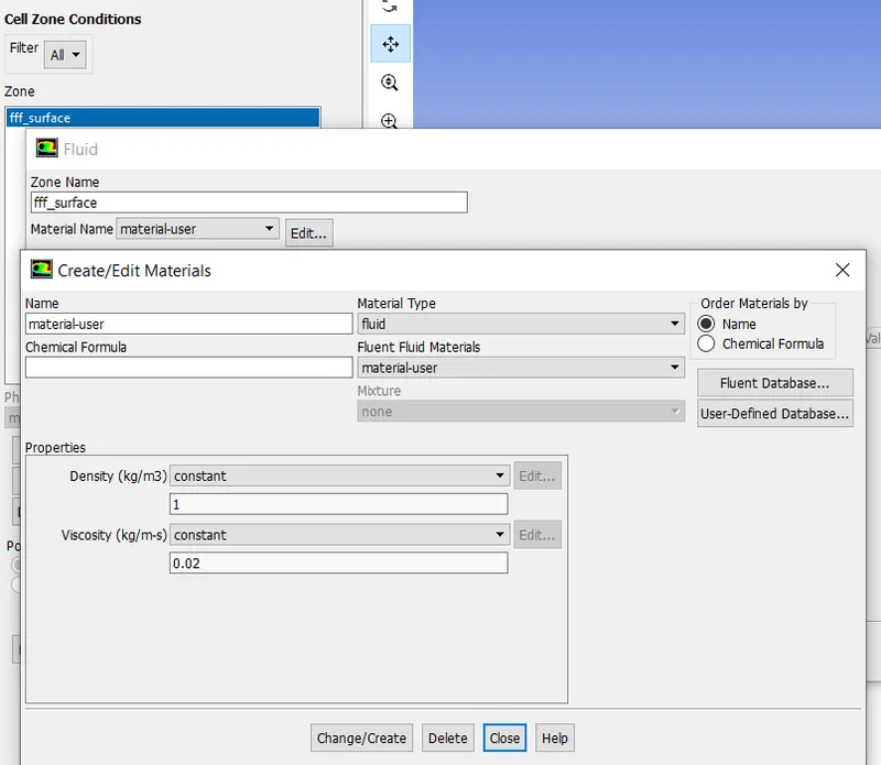Density & viscosity are kept constant.

Boundaries & Intial condition -

Inlet - Velocity type; outlet -pressure type; top & bottom edge -symmetry type; cylinder - wall type.

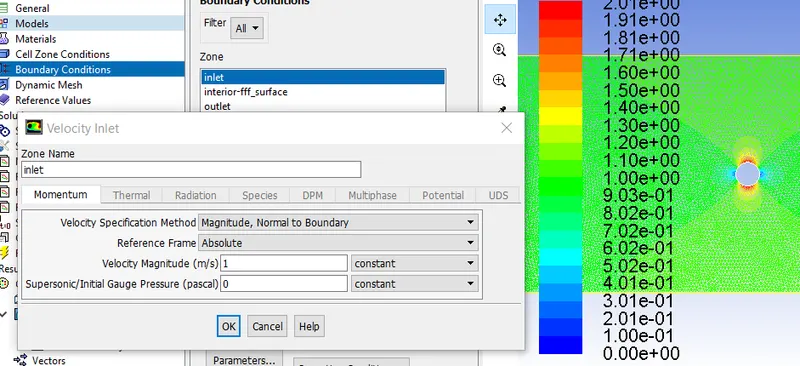
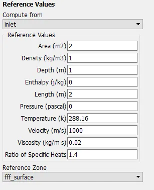
Refernce values - computed from Inlet & kept same values for all cases.

Solving :

Solution methods - Pressure-velocity coupling - SIMPLE scheme is used to discretize & solve the flow problem.

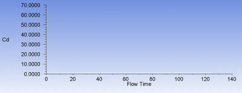
Monitors - 'Cd & Cl' are monitored in the cylinder wall zone & result plots are obtained after calculation.

Report Definitions -

• Surface report of vertex average type is created to obtain velocity at set monitor point.
• Force report of Lift & drag are created to check the co-efficients in cylinder wall zone.

Solution Intialization - Hybrid Intilization is done on all cases.

Postprocessing :

Monitor point - Vertex Average velocity is monitored at this point to further calculate Strouhal No.

contours - Velocity & pressure contours files are created to view in playback or animation

Solution playback animation - Flow variables variation are viewed after result are being obtained.

Results :

a) Steady state solution - Re-100

Inlet velocity = 1 m/sec.

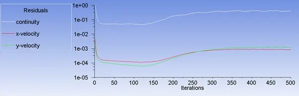
• After 250 iterations Residuals became constant.

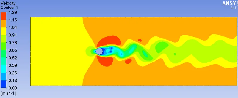
Velocity contour

Pressure contour

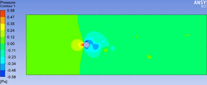
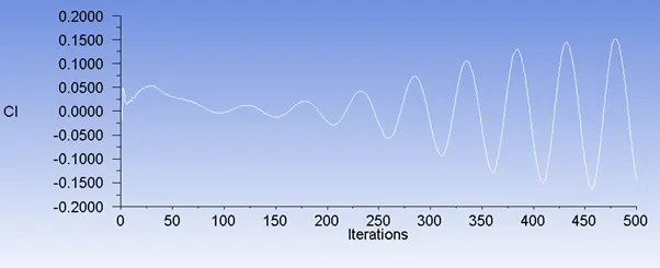
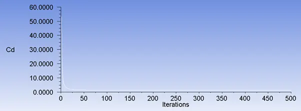
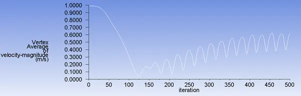
• After 350 iterations ,Vertex average velocity is varying constantly, reached steady state.

b) Unsteady/transient state solution - Re-100

Time step approach details :

Time step size = 0.1

No. of time steps = 1250

Total simualation time = 125sec.

Max. itterations/time step = 20

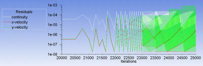
• After 2200 iterations residuals varying within constant limits.

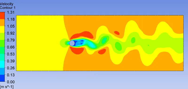
Velocity contour

Pressure contour

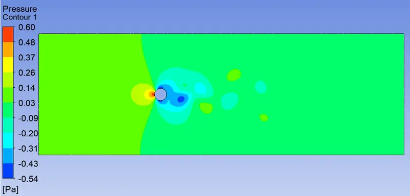
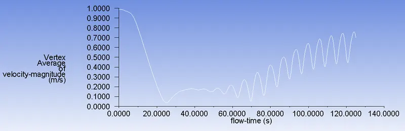
V-vertex = 0.7m/sec

Comments :-

• In both aproaches we can clearly observe the vertex shedding formation of laminar flow behind the cylinder (velocity contour). Steady state simulation took less time compared to transient,but in transient data captured was accurate with respect to flow time.
• To confirm that the solution has converged we can check the residual & Velocity average plots, where either this curves approached straightline or forming repeating pattern.

Strouhal number -

The Strouhal number represents the ratio of inertial forces due to the local acceleration of the flow to the inertial forces due to the convective acceleration.

Basically Strouhal number is associated with the oscillations of the flow. At high Strouhal numbers oscillations dominate the flow while at low Strouhal numbers the oscillations are swept by the fast-moving fluid.At intermediate Strouhal numbers, approximately 0.2–0.3, the well known shedding of vortices downstream of a cylinder takes place.The vortex frequency has been found to depend linearly on the velocity far upstream of the cylinder. The spacing of the vortices is clearly dependent on the Strouhal number and is a function of Reynold's no., where plot of Re vs St shows several pairs of discrete vortices are formed behind the cylinder in staggerd arrangement.

is given by `St = (f*L)/U`

f=shedding frequency

L= characteristic length (Dia of cylinder)

U=flow velocity

Direct calculation :-

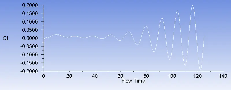
f=2/(110-85)=0.08hz (Cl peaks/flowtime)

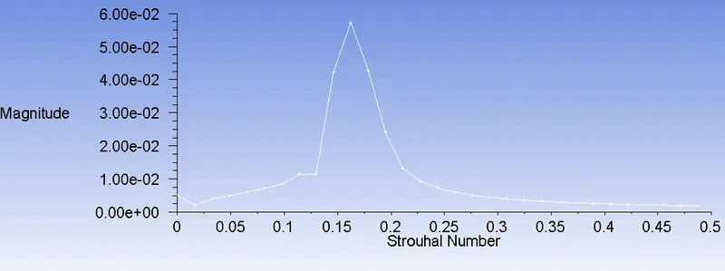
St = (0.08*2)/1 = 0.16

Using FFT function 'lift coeffecient' input file was uploaded to plot strouhal no.

At peak magitude , St.no = 0.16

Part 2 -

a)Finding the coefficient of drag and lift over a cylinder by setting the Reynolds number to 10,100,1000,10000 & 100000

Note : Steady state method solving is done for all cases to compare the results.

	Average values
Reynold's no	Cd	Cl	Average velocity vertex
10	3.327	-0.00055	0.043
100	1.346	-0.144	0.619
1000	0.766	-0.126	7.24
10000	0.515	0.244	71.53
100000	0.506	0.156	714.28

Effects of Cd on Re:-

Stokes Law : Stokes obtained the solution for the pressure and velocity field for the slow motion of a viscous fluid past a sphere. Where he dervied an expression for frictional /drag force excerted on spherical objects with very small Reynold's no.<<1 in a viscous fluid.

`Cd =24/(Re)`

As the Reynolds number increases, flow separation gradually develops, and this corresponds to a change from a regime of flow dominated by viscous effects to a regime of flow dominated by flow-separation effects, with pressure forces far larger than viscous forces. The curve remains straight line until Re<<1. After flow separation established, the curve for Cd shows no relationship whatsoever to Stokes’ law.

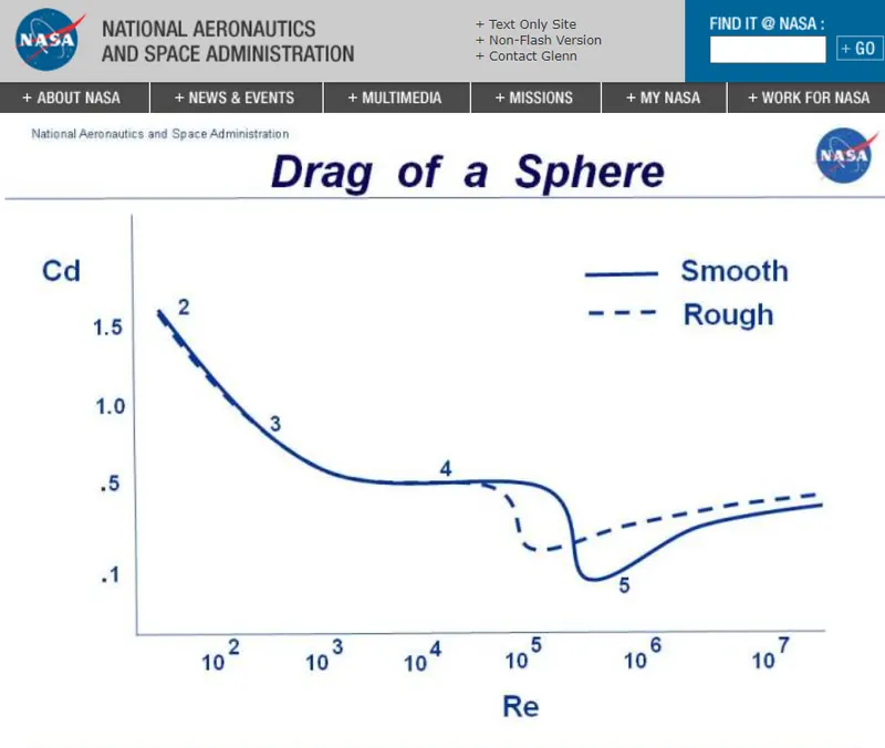
Pressure drag is more signficantly contributes in the blunt body shapes like cylinder/sphere compared to shear drag, because of the pressure difference created b/w front & rear side of cylinder, which is when the flow sepreation occurs creating a wake of re-circulating flow, this creating an further low pressure area behind the body called seperation region results in a large drag force.

• It is evident from the obtained results in the table above at different values 10< Re<1e5, that as Re increases Cd decreases.
• The Cd values are approxly matching to the above Plot from Nasa.(assuming deviations are <5%)
• The drag force reduces significantly in the transition region (`10^5 -10^6`), because when flows starts to become transient it delays the flow seperation from the cylinder wall.
• At the low end of the range, i.e. for Re<100, the flow behind the cylinder is pure laminar, and the vortices remain distinctly shaped even at large distances from the cylinder. The periodic vortices finally disappear at very high values of the Reynolds number, and a turbulent wake forms behind the cylinder.

Co-efficient of Drag

Re -10

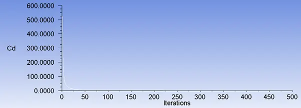
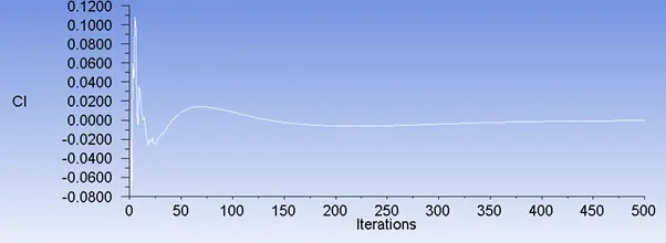
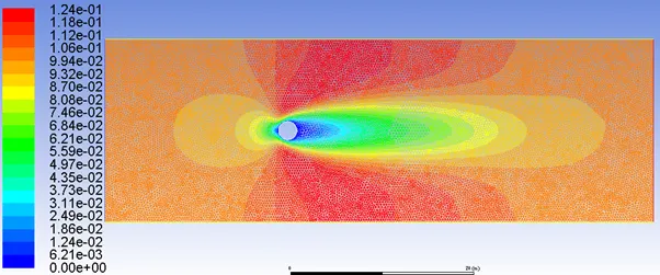
• Flow seperation has occured but there are no such eddies formation.

Re -100

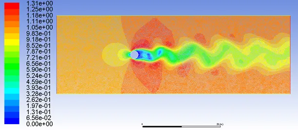
• There is a formation of ring eddy behind the cylinder & the point of separation moves to the side and the ring eddy is pulled indownstream direction and begins to oscillate becoming unstable.

Re -1000

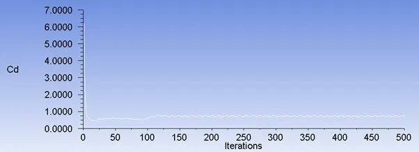
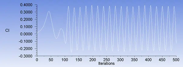
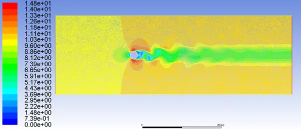
• turbulence begins to develop in the wake of the cylinder and entire wake is filled with a mass of turbulent eddies.

Re -10000

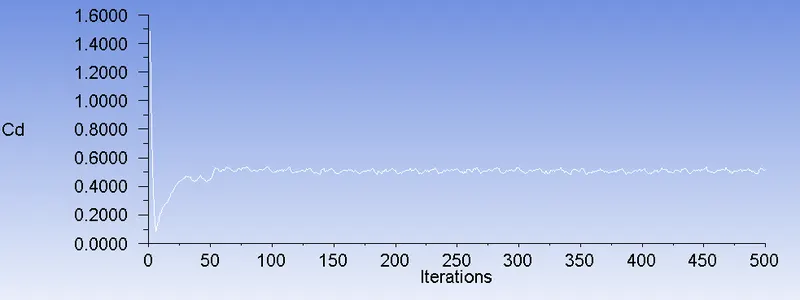
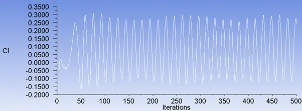
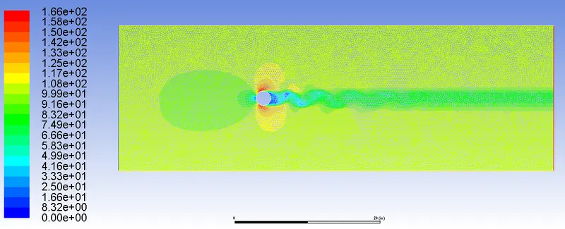
• The pattern of flow does not change much but and there is a fully developed turbulent wake

Re -100000

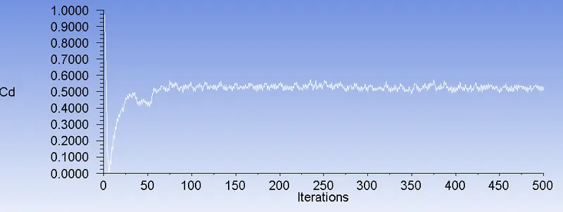
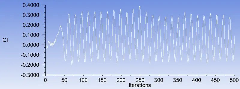
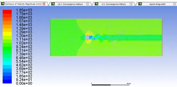
• the boundary layer start to become turbulent before separation takes place, and there is a sudden change in the flow pattern, in which the boundary layer has already changed from being laminar to being turbulent at some point upstream of separation.The wake becomes contracted compared to its size when the separation is laminar, which is the sign of delayed seperation or larger angle of contact around cylinder causing lower Cd.