Challenge

Week 2 - Flow over a Cylinder.

BBalaji K31 Jul 2023

AIM:

To stimulate the flow over a cylinder and to explain the concept of Von Korman Vortex Street. To understand the various flow regimes for the flow passed over a cylinder. And to understand the physical phenomena and the mathematical studies behind the flow regimes. To understand how the flow varies by using steady & transient solver for the same parameters of flow.

THEORY:

Vortex:

Vortex is a region in which the fluid flow resolves around its own axis. Along the axis of the vortex the low pressure is generated. And at the extreme end of the vortex high pressure is generated. The variation in the pressure is generated by the rotational flow with the certain velocity and vice versa

Von Korman Vortex Street:

Prandtl who is the professor of Von Korman in his lab did the research to find out the seperation point when a flow passes over a cylinder using the boundary layer theory. Prandtl appointed the doctorate karl heimenzz to follow the study. But on each and every flow changes, karl identifies unusual oscillation in his channel. Then Von korman did research on this and find out this beautiful phenomenon which is generally called as Von Korman Vortex Street.

If the flow field having any obstruction, flow passes over that obstruction have certain oscillation behind that. This happens due to the velocity of the fluid. When the fluid hits the obstruction high pressure is generated whereas behind the obstruction low pressure is generated. By the mean due to the seperation of fluid happens creates the shear stress layer at the top and bottom of the obstruction also creates the difference in the pressure behind the obstruction.

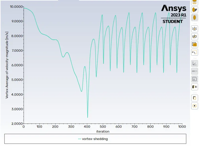
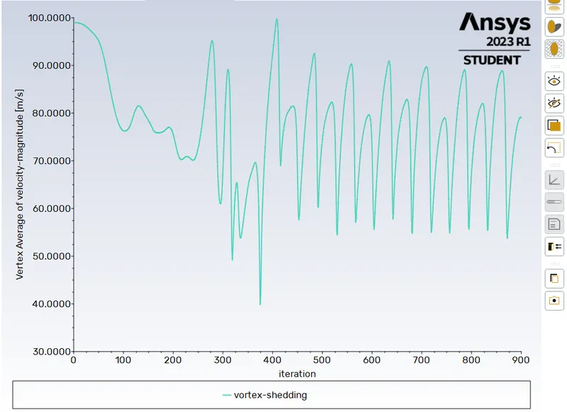
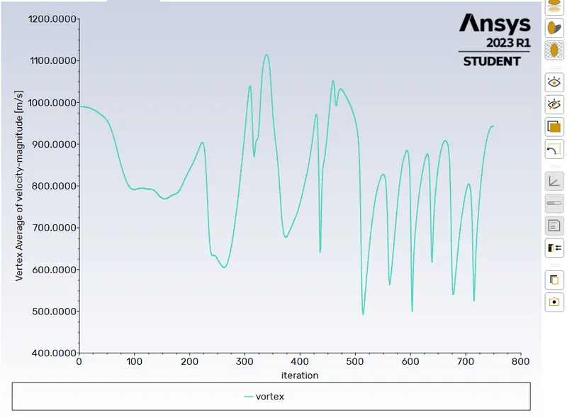
But these changes in pressure difference is mostly oriented by the velocity of the flow field. At a certain flow field where the reynolds number is said to below 40 the identified vortices is found at both the top and bottom. At the range of 40<Re<200 Laminar vortex street observed. Then vortex shedding will happen if the velocity is further increased.

At a certain velocity the shear forces at any one of the end will converge into the wake region where the lower pressure is found, due to that vorticity occurs. The converged shear forces seperates in to three form and will produce vortices and also disturb the shear force at the opposite position.The disturbed shear force then converged into the wake region creates another vortices which will follow the previously generated vortices. This phenomena is known as Vortex Shedding. This is why the vortices produced in von korman vortex street are provided at a spacing ratio.

INTRODUCTION:

In this project, we are going to analyse the von korman vortex street for the following parts

PART I:

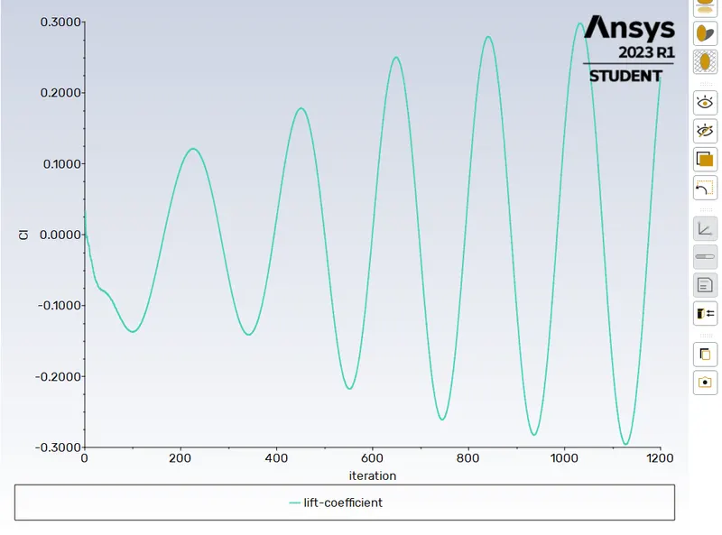
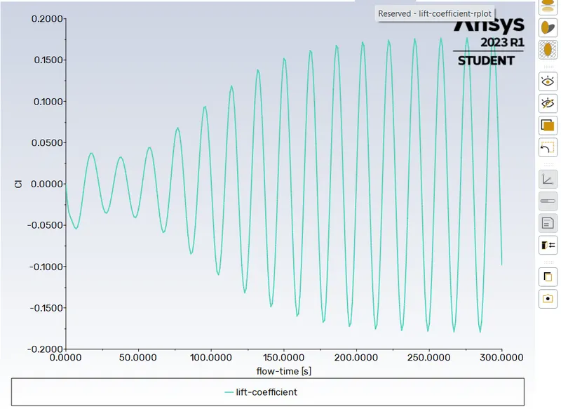
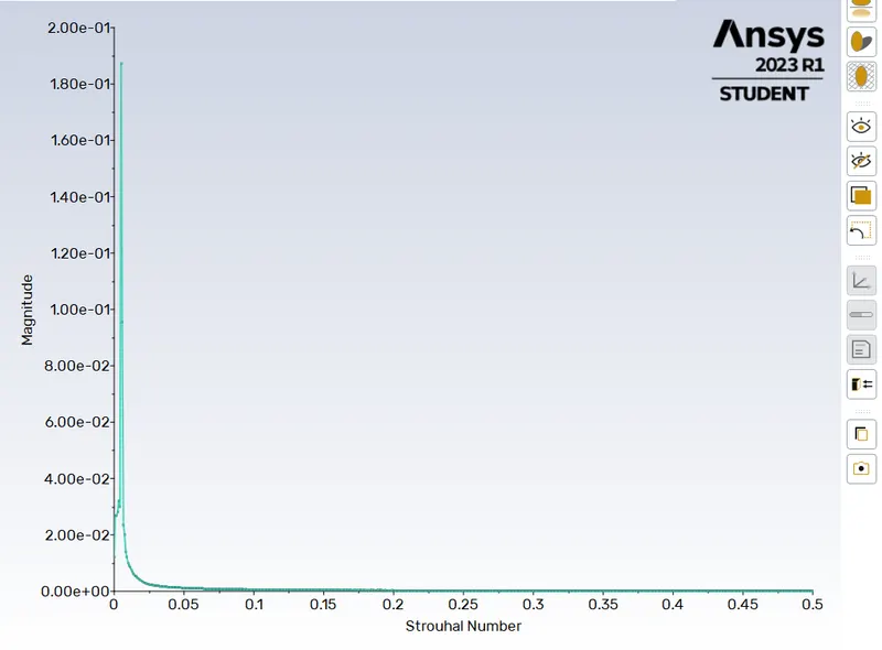
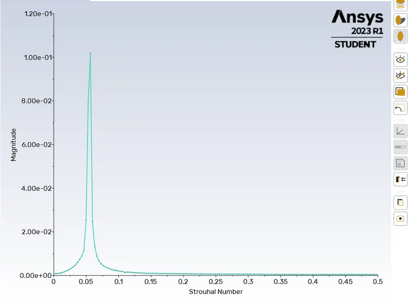
Simulate the flow with the steady and unsteady case and calculate the Strouhal Number for Re= 100.

PART II:

Calculate the coefficient of drag and lift over a cylinder by setting the Reynolds number to 10,100,1000,10000 & 100000. (Run with steady solver)
Discuss the effect of Reynolds number on the coefficient of drag.

PROCEDURE:

Geometry creation:

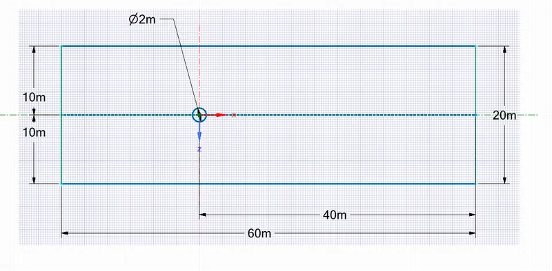
According to the problem stated, sketch is drawn in the space claim. Then using the PULL command surface is generated over the drawn sketch. The entire sketch is created by keeping the wall centre as an axis point.

Meshing:

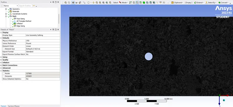
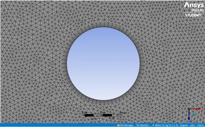
The geometry is loaded in the meshing area. Initially the automatic meshing is done, which contains quadilateral shape. Then using the Sizing ------> Face Sizing command, converted all quadilateral mesh to the triangular mesh.

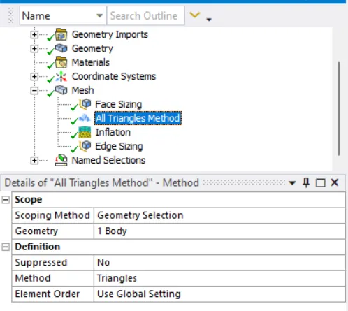
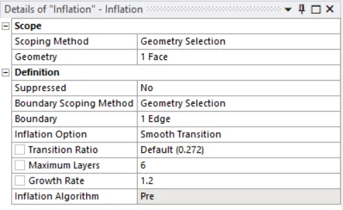
Then using the face sizing option to reduce the element size to capture the effect accurately. Then the inflation layer is used near the wall. The inflation layer produces the mesh layer which will replica the geometry shapes, thus the smooth transition occurs at the wall.

Problem Setup:

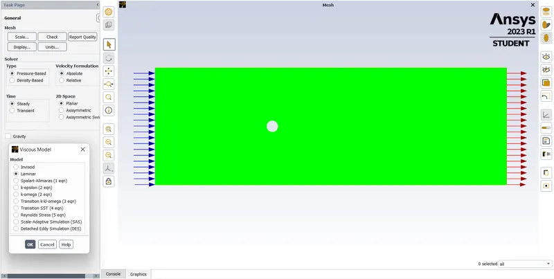
Parameters taken in Part I and Part II:

Model : SIMPLE

Viscous model : Laminar

Solver : Pressure-Based

Velocity formulation : Absolute

Time : Steady for Re 10,100,1000,10000,100000 & transient for Re 100

Meshing : Manually generated.

Dynamic Viscosity of the fluid : 0.02 Kg/ms

Working fluid : Air

Density of the fluid : 1 Kg/m3

PART I:

Case I - Steady solver with Re - 100:

Using the reynolds number equation we can find the velocity for this particular reynolds number.

`Re underset(L) () = (U L rho)//mu`

`U = (Re .mu)// (L.rho)`

U = (100x0.02)/(2x1)

U = 1 m/s

Case II - Transient solver with Re - 100:

Using the reynolds number equation we can find the velocity for this particular reynolds number.

`Re underset(L) () = (U L rho)//mu`

`U = (Re .mu)// (L.rho)`

U = (100x0.02)/(2x1)

U = 1 m/s

Lets compare the results for the above two cases,

Scaled Residuals:

For Re - 100 Steady Solver For Re- 100 Transient solver

The residuals are the imbalance of potential factor in the equation due to the interative operation in the CFD. Basically residuals are the errors of solving the governing equation for each mesh in the solving domain. CFD have to solve the solution for each and every generated mesh quantity. While piling up the results residuals may found. In the initial iteration we can see the variation of residuals in maximum because when the iteration is being solved, the outcome results of the first iteration is the input function of the further iteration. When the residuals are of complete zero, then the solution is considered to be as solved and the convergence is reached.

But in the practical problems the zero residuals is not even possible to obtain. But as per the mathematician and physicist concern, whenever there is of zero residuals then only they consider the solution is being solved. But the engineering perspective is different , we are looking for the constant residuals over the time. If it is achieved then we assume the solution is converged. In CFD solver, for each and every transport equation the residuals value is predefined. When the solution reaches the pre defined value the iteration is stopped and shows us the result that the solution is converged.

Factors to be considered to check for the divergence:

For every problem we have to solve the transport equation for obtaining the solution. Depending upon the problem choosen continuity equation will be there. And the CFD solver has the scaled residuals option for the continuity equation. We have to check in the continuity equation value whether the value reaches the constant factor for large number of iterations. But in some cases, we have to look for the solution required. Lets assume in our problem we have to check for the vortex average at the monitor point and also the lift coefficient at the wall. In that particular graph we have look for the constant value for the certain amount of the iteration. If it keeps constant over a particular period of iteration then we can assume that the solution is being solved and it is converged. So by these two values we can justify whether the divergence is occured or not.

Vortex Shedding:

For Re - 100 Steady Solver For Re - 100 Transient Solver

In some cases, we cant able to consider the solution is converged by seeing the residuals as it may vary in a non-similar way. For that based upon the required result we put monitor points in a certain area and observe the flow field with respect to our results. Then we have to observe the common patterns in those points or the constant value, then with that value we will conclude whether the solution is converged or not.

Drag Coefficient:

For Re - 100 Steady solver For Re-100 Transient Solver

In this for steady solver, the drag coefficient is common after the 80 iterations, whereas the residuals are in still keeps on increasing. So for that we have to run more iteration to identify the solution is converged or not. By that consideration we have to consider the other factors as well like vortex shedding and lift coefficient.

Lift Coefficient:

For Re - 100 Steady solver For Re - 100 Transient solver

By viewing the lift coefficient plot for the steady solver after the 600 th iteration the residual values are in constant phase, whereas the lift coefficient is also in the increasing span. For that we have to look for the residuals in this Re-100 steady solver. But for transient the residuals are in varying abnormally, But after 175 flow times the flow pattern in lift coefficient seems to be in a same phase. So with that reference we can stop our iteration by confirming that the solution is converged.

Strouhal Number:

For Re - 100 Steady solver For Re - 100 Transient solver

Strouhal number is a dimensionless number used to describe the oscillating flow mechanism. It is described as the ratio of the intertial forces due to the local acceleration to the inertial forces due to the convective acceleration. It is given by the formulae

`Sr = (fxx L)/U`

Where f- frequency of vortex shedding here

L - Chareacteristic length(Wall diameter)

U - Flow velocity

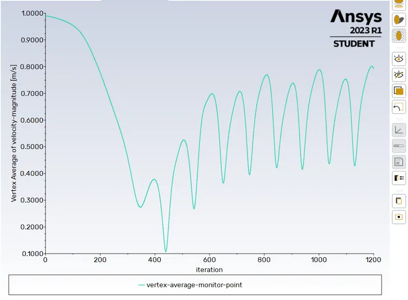
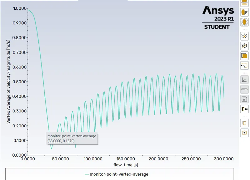
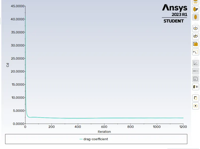
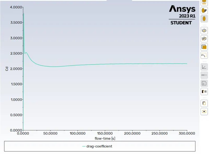
PART II:

Case I - Steady solver with Re - 10:

Using the reynolds number equation we can find the velocity for this particular reynolds number.

`Re underset(L) () = (U L rho)//mu`

`U = (Re .mu)// (L.rho)`

U = (10x0.02)/(2x1)

U = 0.1 m/s

Case II - Steady solver with Re - 100:

`Re underset(L) () = (U L rho)//mu`

`U = (Re .mu)// (L.rho)`

U = (100x0.02)/(2x1)

U = 1 m/s

Case III - Steady solver with Re - 1000:

`Re underset(L) () = (U L rho)//mu`

`U = (Re .mu)// (L.rho)`

U = (1000x0.02)/(2x1)

U = 10 m/s

Case IV - Steady solver with Re - 10000:

`Re underset(L) () = (U L rho)//mu`

`U = (Re .mu)// (L.rho)`

U = (10000x0.02)/(2x1)

U = 100 m/s

Case V - Steady solver with Re - 100000:

`Re underset(L) () = (U L rho)//mu`

`U = (Re .mu)// (L.rho)`

U = (100000x0.02)/(2x1)

U = 1000 m/s

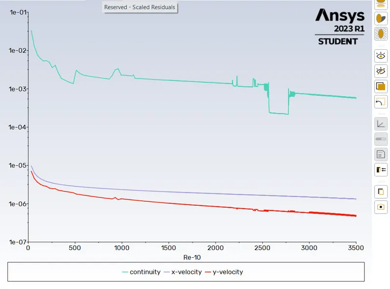
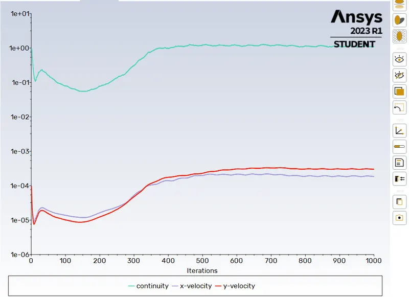
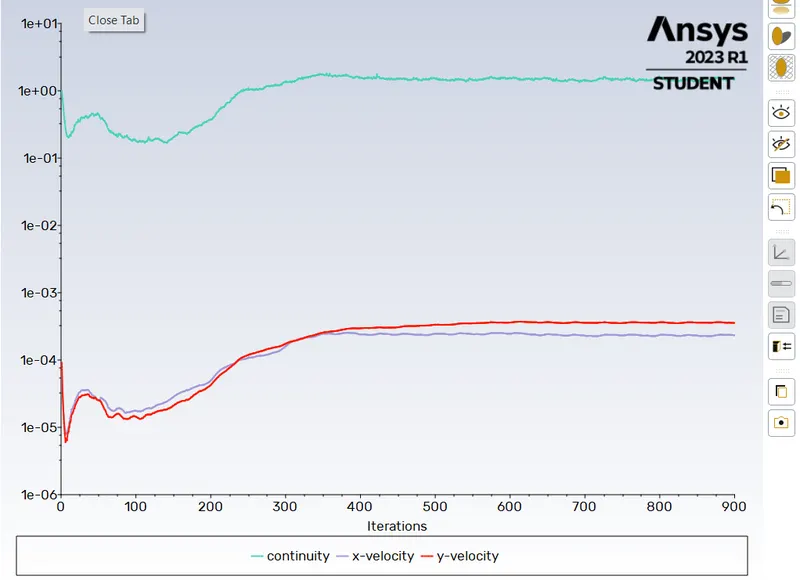
Scaled Residual Plots:

Re - 10 Re - 100

Re - 1000 Re - 10000

Re - 100000

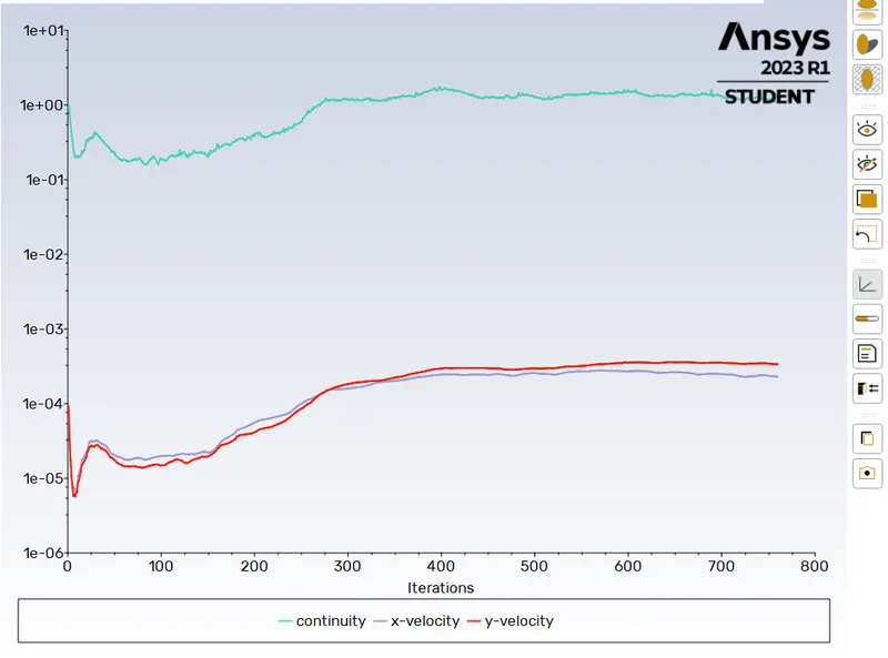
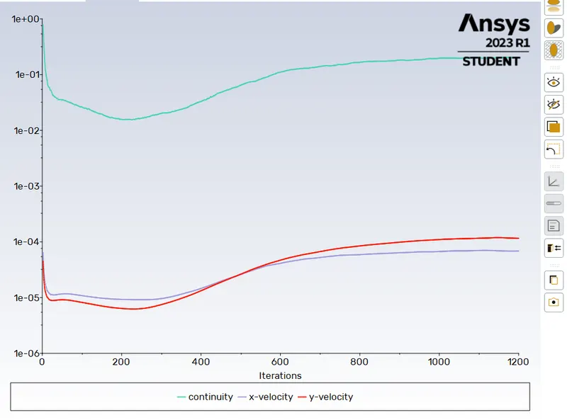
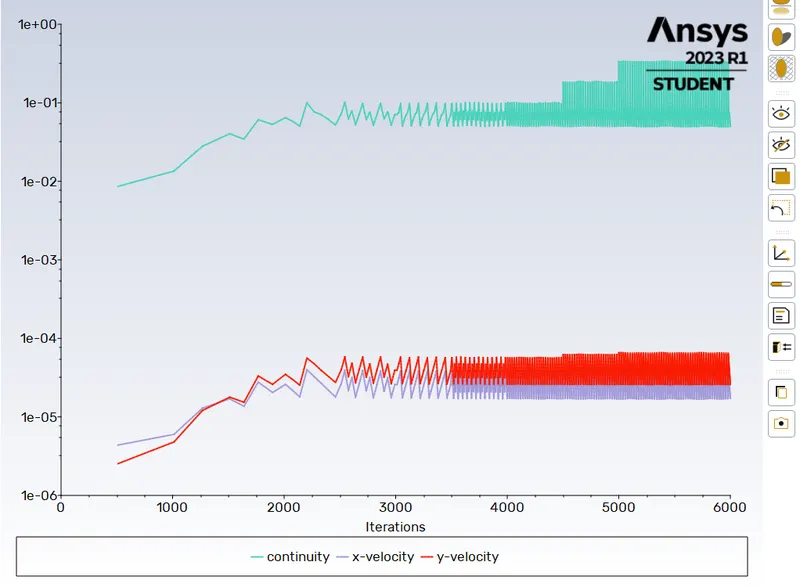
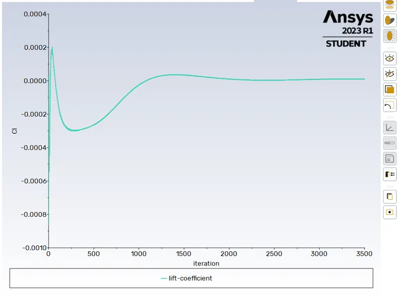
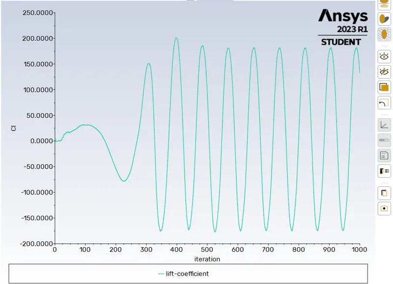
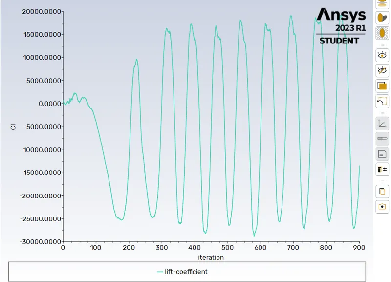
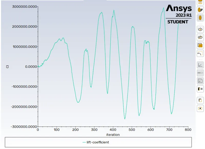
In this project the most of the convergence is observed in the residual plot as well as the lift coefficient plot. Because after the certain iteration the continuity is become constant and no major deviation in observed for the cases with highest reynolds number.

Vortex Shedding:

Re - 10 Re - 100

Re - 1000 Re - 10000

Re - 100000

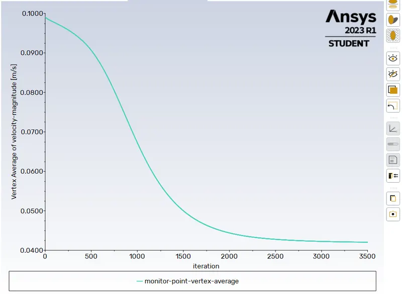
For the Re-10, the convergence is observed by the vortex shedding plot. We can note that after 2600th iteration the plot value are constant and there is no deviation.

Drag Coefficient:

Re - 10 Re - 100

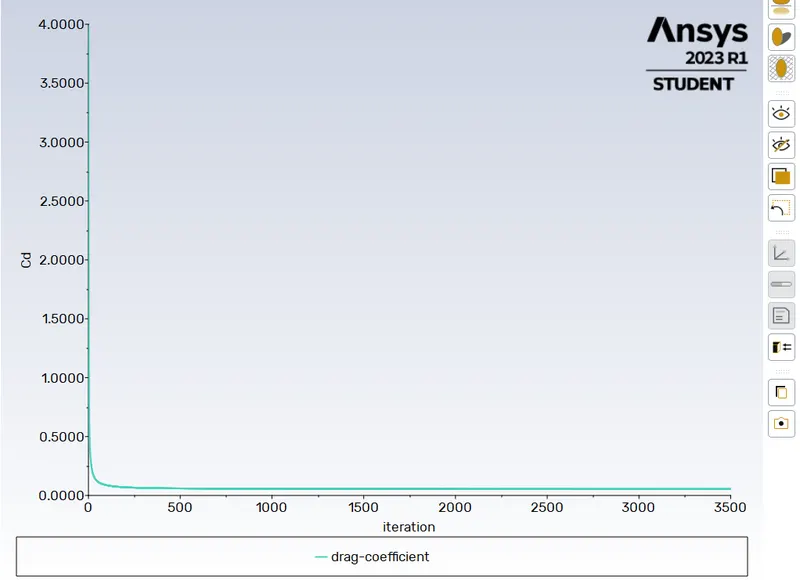
Re - 1000 Re - 10000

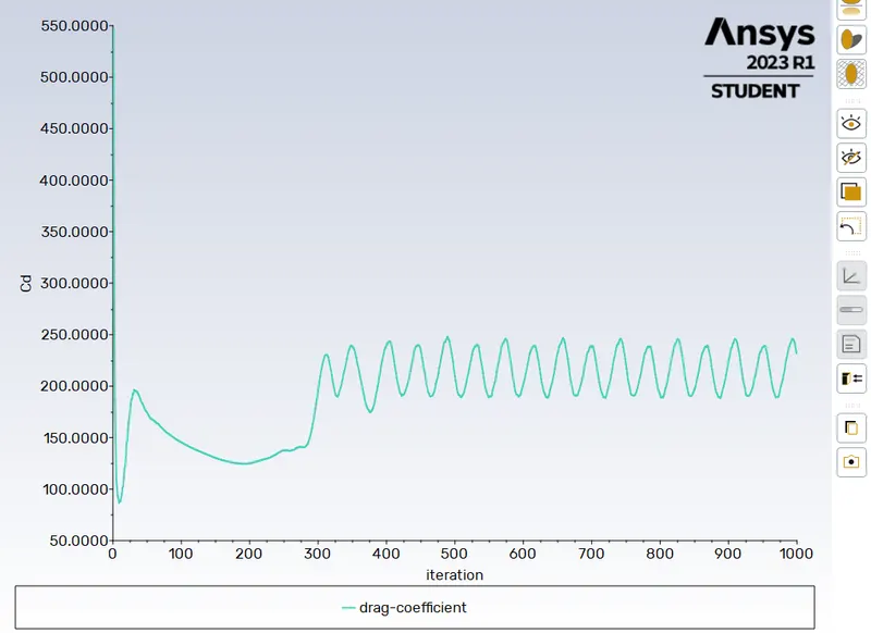
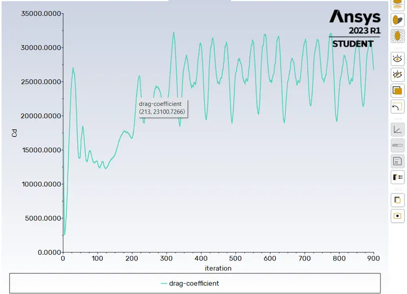
Re - 100000

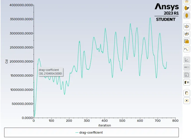
Lift Coefficient:

Re - 10 Re - 100

Re - 1000 Re - 10000

Re - 100000

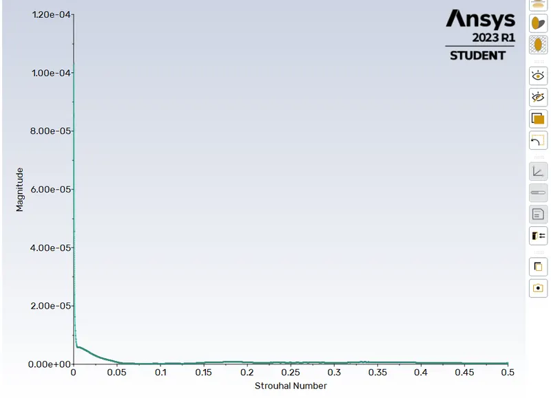
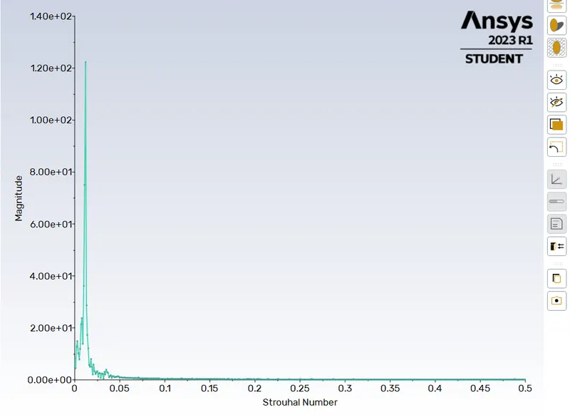
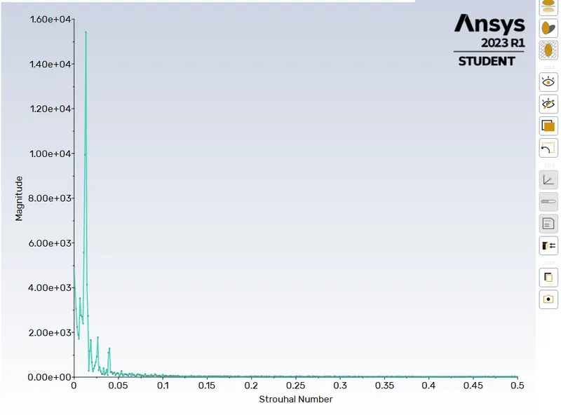
Strouhal Number:

Re - 10 Re - 100

Re - 1000 Re - 10000

Re - 100000

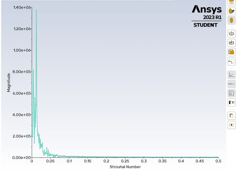
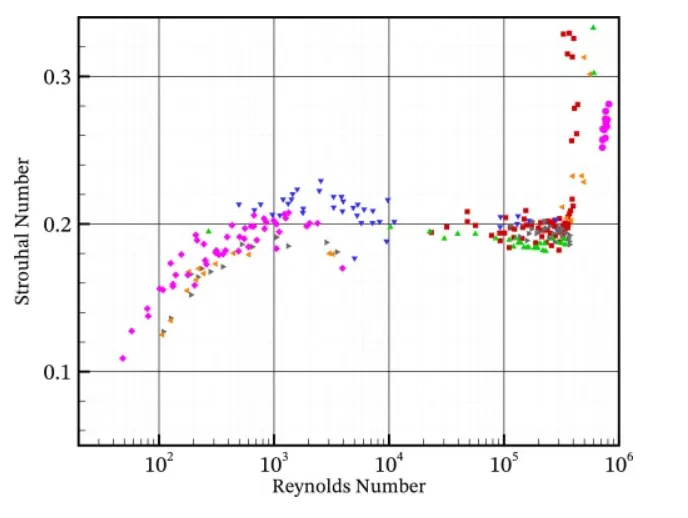
Higher the strouhal number the oscillating field dominates the flow, Lower the strouhal number the velocity of the fluid dominates the flow field. And reynolds number has a direct relation with the strouhal number. Increasing in the reynolds number strouhal number is also increasing. For the 10^2 < Re < 10^5, we observe the strouhal number values are in and aroung 0.2. To the further increasing in the reynolds number sudden peak rise found in the strouhal number.

LEARNING OUTCOMES:

Basic understanding of how to create the geometry in the space claim
Learned how to use the different methods of meshing depending on the flow field and the geometry.
Understanding the concept of Vortex and vortex shedding.
Understanding the phsyics behind the Von Korman Vortex Street.
Got knowledge on how to check for the convergence and got the idea of what residuals are.
Analysed the solution for Steady and Transient solver and observed the variation in each solver.
Got the understanding of how the vortices are increasing as the reynolds number is also got increased.

RESULTS:

Thus the flow over a cylinder is done by adjusting various reynolds number and the phenomena of Von Korman Vortex Street also observed.

Week 2 - Flow over a Cylinder.

Ship work like this
in your own course.

Talk to a career counsellor

Ship work like thisin your own course.

Talk to a career counsellor

Ship work like this
in your own course.