Week 2 - Flow over a Cylinder.

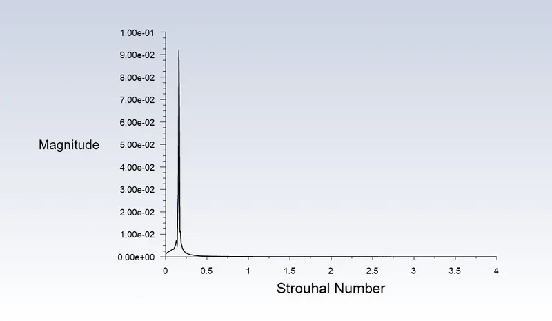
Aim :- Simulate the flow over the cylinder and calculate the Strouhal Number for a given problem using workbench-fluent under steady and unsteady case for Re= 100. And explain the phenomenon of Karman Vortex Street.

Also calculate the coefficient of drag and lift over a cylinder for Reynolds number 10,100,1000,10000 & 100000 under steady state condition. Discuss the effect of Reynolds number on the coefficient of drag.

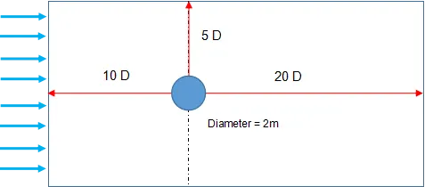
Expected results:

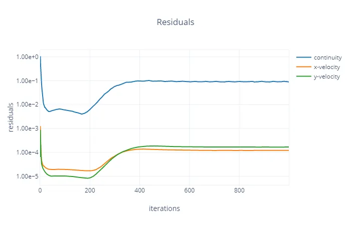
• In both approaches, show that the flow has converged. That is, what quantities or plots need to be looked at to determine that the flow has converged?
• Plots of the coefficient of drag and lift.
• Create an animation for any one case to show the vortex shedding behind the cylinder.
• Plots to show vortex shedding behind the cylinder.
• Mention the referred material (Reference Paper or Fluid Mechanics Textbook) at the end of the challenge submission page

Introduction :-

Flow over a Cylinder :-

The flow past a two-dimensional cylinder is one of the most studied of aerodynamics. It is relevant to many engineering applications. The flow pattern and the drag on a cylinder are functions of the Reynolds number.

Reynolds Number(Re) :-

The Reynolds number for a flow measures the ratio of the inertial to viscous forces in fluid flow around a body.
where,
ρ= Desity of medium
V= Velocity of the medium
d= characteristic length
μ= dynamic viscosity
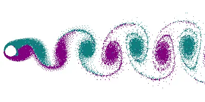
The range of Re values will vary with the size and shape of the body form in which the eddies are being shed, as well as with the kinematic viscosity of the fluid. over a sizeable Re range eddies are shed continuously from each side of the boundary, forming rows of vortices in its wake. The alternation leads to the core of a vortex in one row being opposite the point midways between two vortex cores. In the other row, giving rise to the distinctive pattern shown in the picture. Ultimately, the energy of the vortices is consumed by viscosity as they move further downstream, and the standard way disappears.

According to study over flows with Rynold Number

for external flow when

Re ≤ 2 x 105 Then its a Laminar flow.

Re > 5 x 105 Then its a Turbulent flow.

The flow seperation occurs fue to change in pressure which causes the drag and lift

For laminar flow the wake region should be btw 75° - 85°

For Turblulent Flow the wake region will lie btw 115° - 125°

Vortex Shedding :-

Vortex shedding is an oscillating flow that occurs when a fluid such as air or water flows past an obstacle body atspecific velocities, depending on the size and shape of the body. In this flow, vortices are created at the rear end of thebody. the flow detaches periodically from either side of the body forming a VON Karman vortex. The fluid flow past the object creates alternating low-pressure vortices on the downstream side of the object. The object will tend to move toward the low-pressure zone.
Suppose the object structure is not mounted rigidly and the frequency of the vortex shedding matches the resonancefrequency of the structure. In that case, the structure can begin to resonate, vibrating with the harmonic oscillations driven by the energy of the flow. This vibration is the cause of the overhead power lines humming in the wind, and the fluttering of automobile whip radio antennas at some speeds. Tall chimneys constructed of thin-walled steel tubes can be sufficiently flexible that, in airflow with speed in the critical range, vortex shedding can drive the chimney into violent oscillations that can damage or destroy the chimney.

Strouhal Number (St) :-

A strouhal number is a dimensionless number describing oscillating flow mechanisms.
The Strouhal number is often given as

St = (ω ⋅ d)/u

where,
ω= frequency of the vortex shedding
d= characteristic length
u = flow velocity

Procedure :-

Spaceclaim Geometry Procedure :-

• We will first open Spaceclaim and create a sketch in a Plane x-y as given in the problem statement , in which the circle in represents the cylinder walls and the larger rectanglle represents the wind tunnel.
• Select circle tool to to draw a circle at the origin.
• use construction lines to find out the point at the left side from where we can draw a rectangle of the same dimensions given in the problem statement.
• 
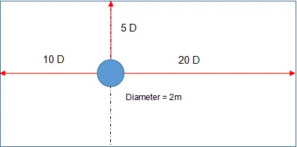
• Now, use Rectangle tool to draw a rectangle tool to create a rectangle of given size and delete the construction lines..
• Now, use pull Command to convert this 1-D sketch into a 2-D geometry.
• Now, Select the inner circle and delete it.
• 
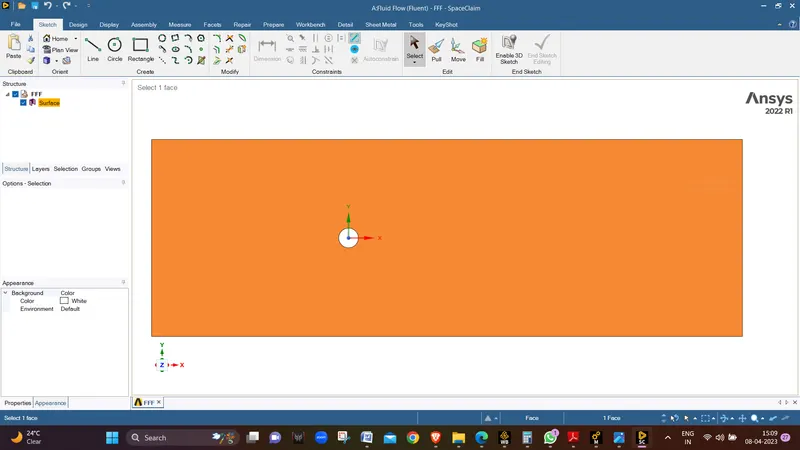
• Close spaceclaim and open Meshing module.

Meshing Procedure :-

• Open Meshing module by performing a double click on Mesh button in the fluent module.
• Once Meshing window opens we will perform a default mesh
• 
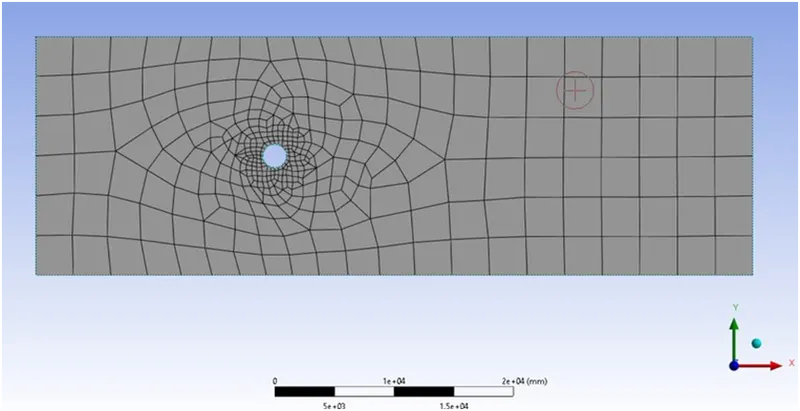
• now we can see thatwe are unable to capture the geometry properly so we will go for a smaller element size lets thae the element size as 250 mm and update the mesh.
• 
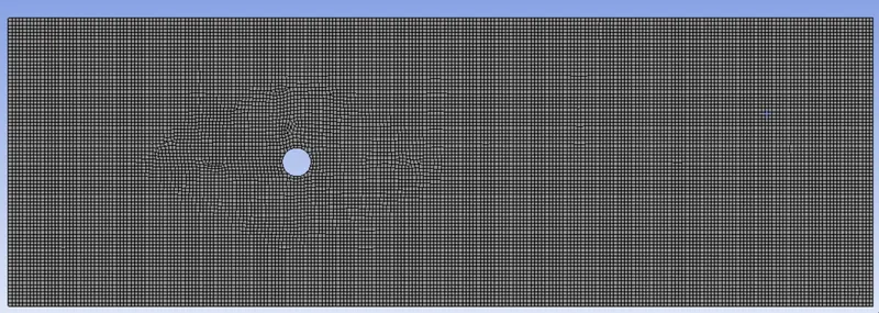
• Now we can see that we have got a refined mesh but when we zoom in on the cylinder area wecan see that we now also have the distorted circle.
• 
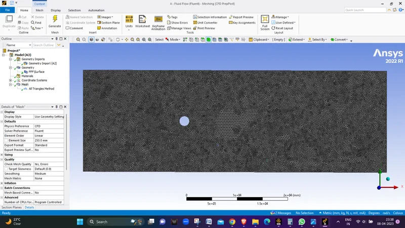
• Now we will go with the refinement of mesh using triagle elements instead of structured elememts by adding methods to the mesh and selecting triangle elements and updating the mesh.
• 
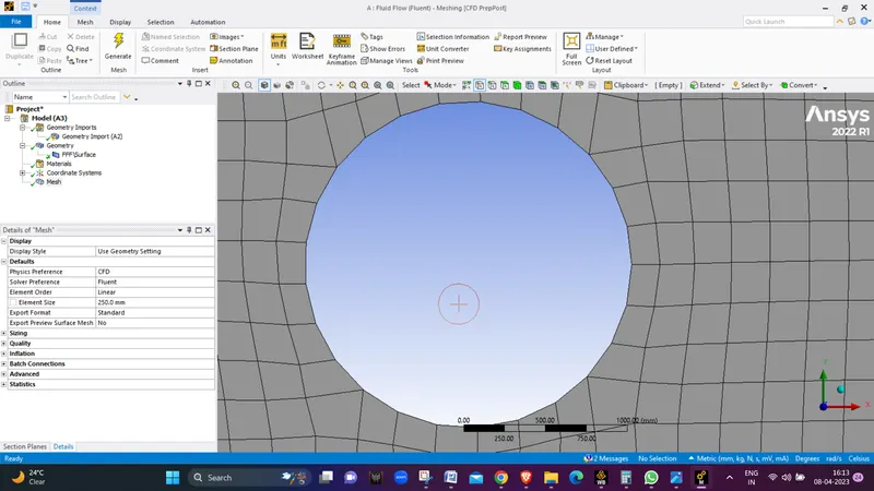
• This is a much refined mesh as compared to structured ne but when we zoom in we find the same circles not in proper shape so we will now give sizing at the edge of circle with number of divisions as 100.
• 
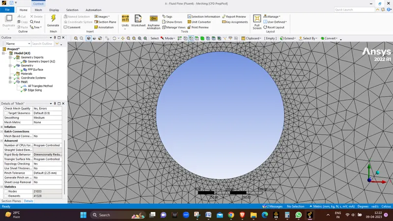
• Now we can see that the circle is in proper shape.
• Now we will add inflation layers but before adding inflation layers lets see what are infltion layers , why we use them and what is the maximum hight we should use for the inflation layer with growth rates of layers.

The image attached shows the boundary layer development. We first start in the laminar region, then transition to the turbulent region. Nearthe wall, due to the viscous forces, the velocity is dragged to zero and as the boundary layer develops, the velocity will reach free-streamvelocity. This is termed as the no-slip condition.

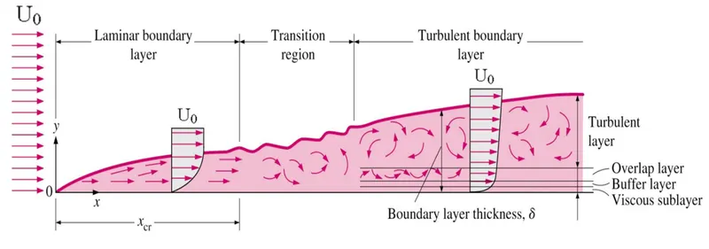
We can use the no-slip condition if we know the flow is completely laminar. This would mean that we are resolving the flow in the laminarregion whatever the grid size. This, however, doesn’t hold if the flow is turbulent. Turbulent flows have a smaller laminar region near the walland if we are to resolve the gradients at such a small region, we’d need a very small grid size.

This is where the y+ value comes in handy. The y+ value is a non-dimensional term that can be used to understand how coarse or fine ourgrid is. This can then be used to determine if wall functions need to be used or not. From the image attached above, we need to either be inthe viscous sub-layer or the turbulent region.

If we were in the viscous sub-layer, that would mean a y+ of less than 10 and if we were in the turbulent region, it would mean a y+ ofgreater than 30. This is very significant in our making the decision of using or not using a wall function.

Before that, let us understand how y+ is calculated and how wall functions affect this calculation.

y+ =y ⋅u_t / ν

where y is the distance from the wall and u_t is the frictional velocity. Knowing

u_t = √(τ_w /ρ)

where τ_w is the wall shear stress which is given by,

τ_w = (C_f ⋅ ρ ⋅ U²_∞ ) / 2

where U_∞ is the free stream velocity and C_f is the skin friction coefficient which is given by,

C_f = 0.0576 ⋅ Re_d^1/5

For a desired y+ value, we can calculate the wall distance or first cell height.

• 12 inflation layers with first layer thickness = 5mm and a growth rate of 1.2, over the edge of circle to capture the flowover cylinder efficiently.
• 
• 
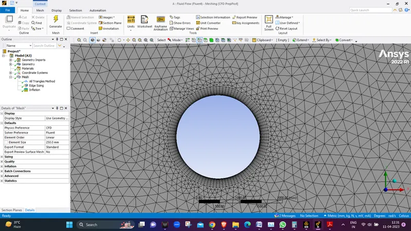
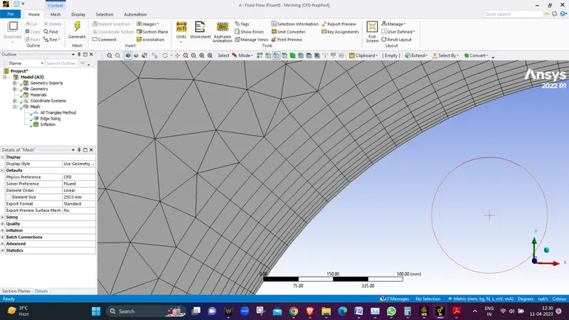
• We have 42020 element in the mesh .

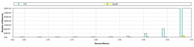
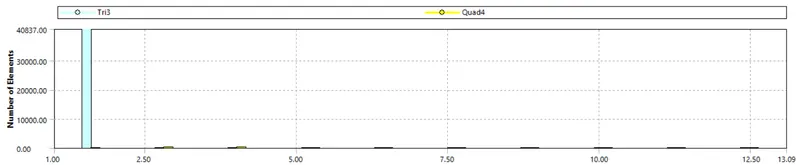
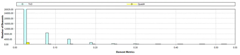
• Following are the Qualaity Criterias :

1. Orthogonality :-
2. Aspect Ratio :-
3. Skewness :-

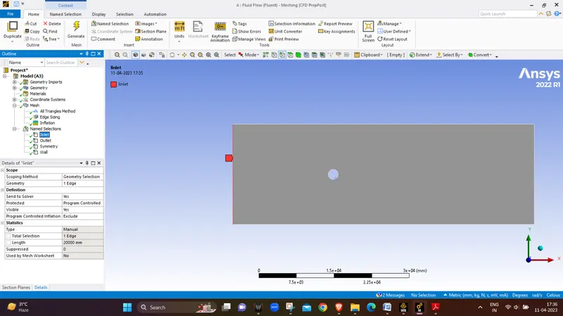
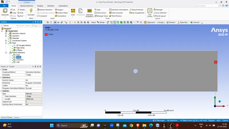
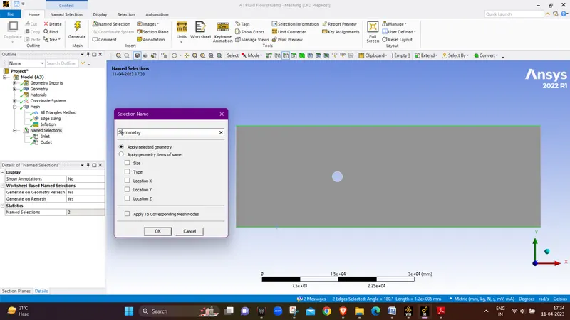
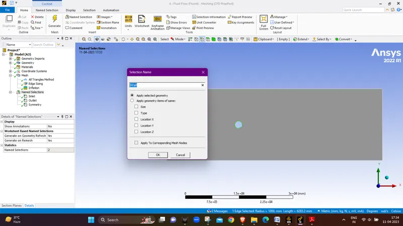
• Now we will assign the boundaries names INLET ,OUTLET, WALL ( Cylinder Edge ) and SYMMETRY ( lengths of cylinder parallel to the flow ).
• INLET
• 
• OUTLET
• 
• SYMMETRY
• 
• WALL
• 
• As we have completed with the assigning the boundaries now we can move to the Solver step.

Solver Setup :-

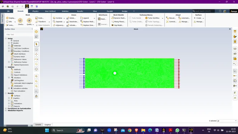
• We will now open Setup to give Initial boundary conditions. On opening setup we will find this grafic window showing inlet with blue arrows and outlet with Red arows and the green area is the wind tunnel area where the aitr flows over the cylinder and the circle in center representing the Cylinder walls.
• 
• We will give the following setting to the setup before running the simulation.
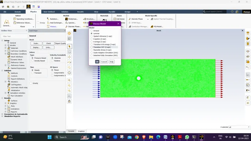
• Select Laminar flow inside the viscous model under physics menu.
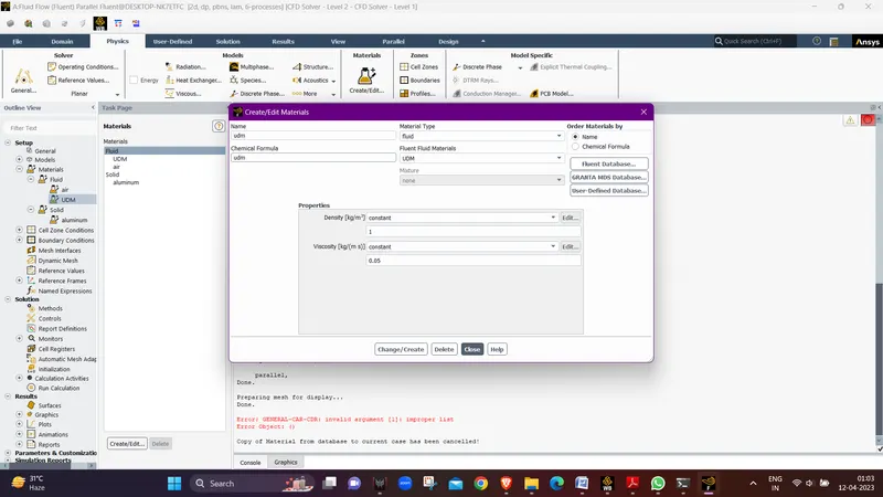
• Now we will material as user define material giving density value as 1 kg/m³ and viscosity as 0.05 kg/(ms).
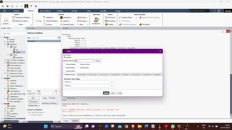
• Assigning the cell zones(fluid domain) material as UDM and delete air from the materials tab.
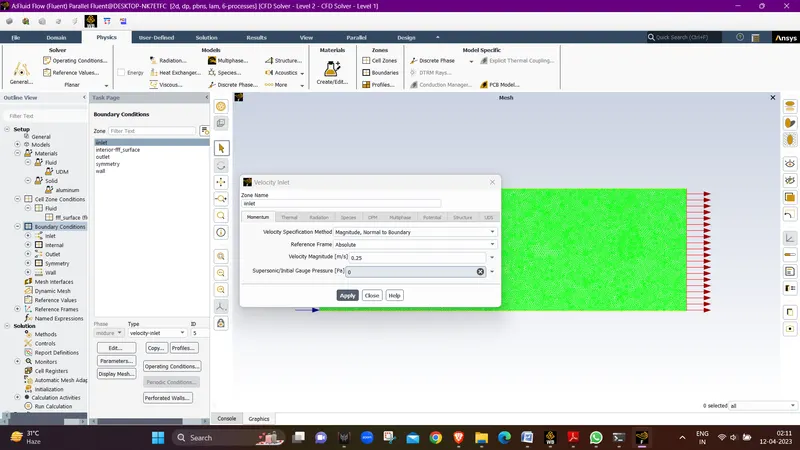
• Giving the inlet boundary condition. We give the inlet velocity as 0.25 m/s for Re=10. and the values change with the Re value respectively for each it is calculated as follows:

  Re = (ρ ⋅ V ⋅ d) / μ

  10 = (1 ⋅ V ⋅ 2) / 0.05

  V = 0.25

  

• we will now assign the report definations for plots in the results one is drag and another is lift.

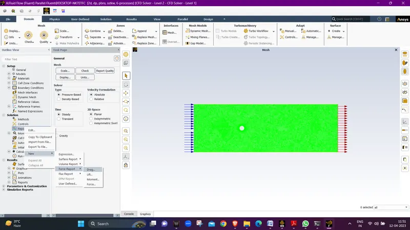
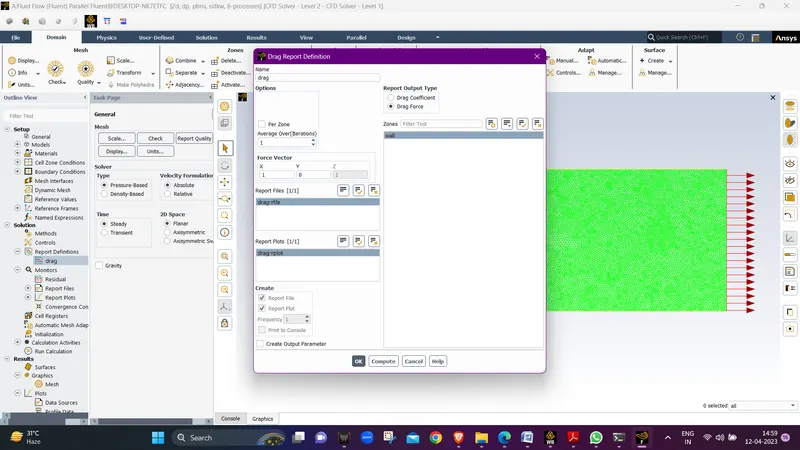
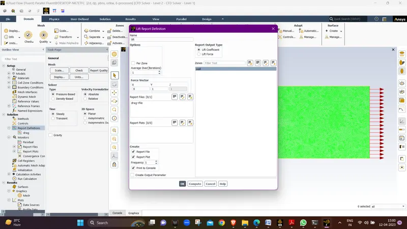
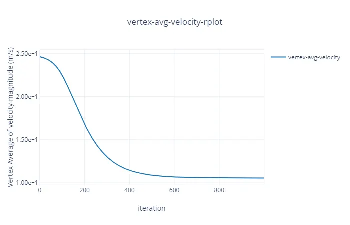
• Now we will create a monitor point to study the vertex average velocity at a point

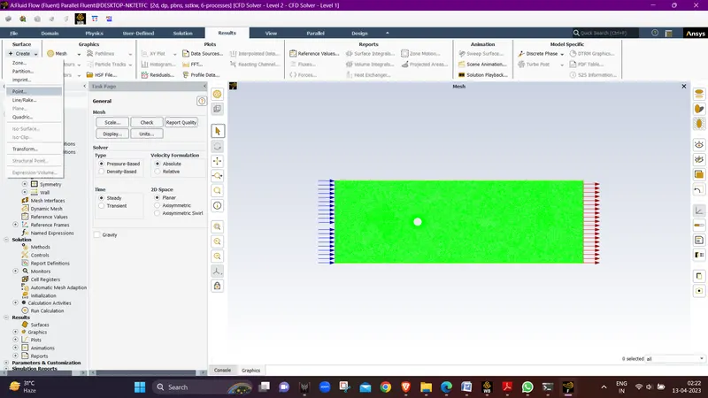
• We will make the point around 4d distance from the cylinder in X direction and d is Diameter of the cylinder which means 8m.

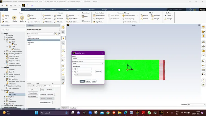
• We will now setup the reference values first.

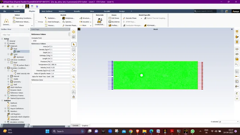
• We will use simple scheme for the methods in the solution tab

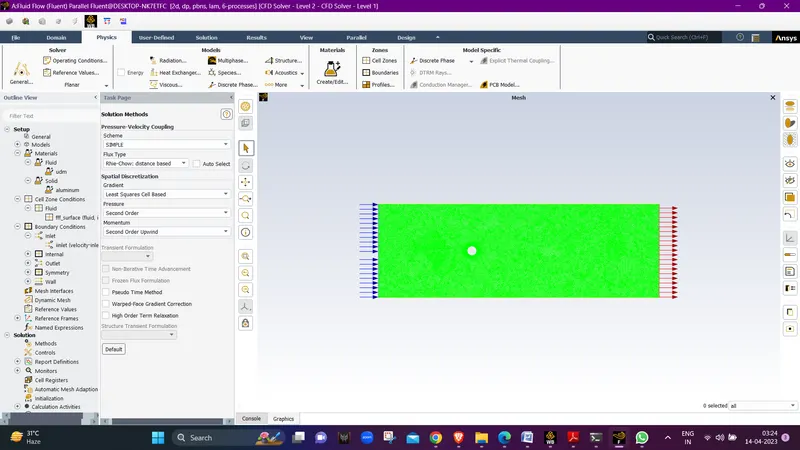
• Now we can define an animation to capture the above contour after every iteration and then form an animation at the end of the simulation.

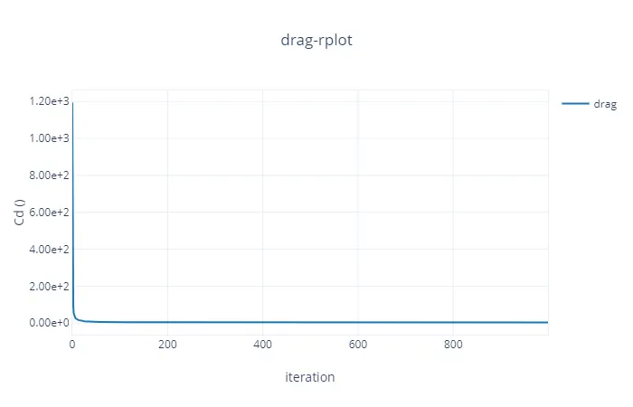
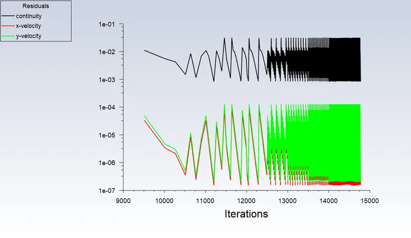
• After this we can simply give run calculations for 500-1000 iterations depending on the case and the no. of iterations it takes for the drag-plot to converge.

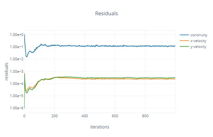
• NOTE: we need to remove the convergence criteria of scaled residuals as they may converge even before the drag value converges

RESULTS :-

PLOTS:

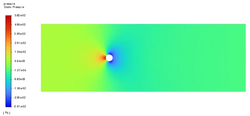
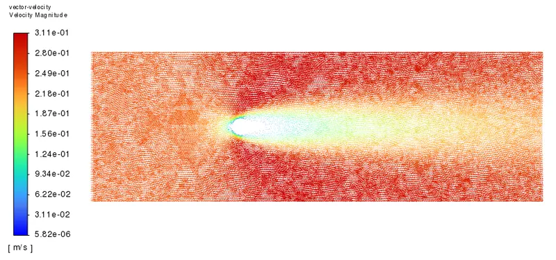
• CASE-1: Re=10, Inlet velocity=0.25, Steady-state solver

Scaled Residuals :-

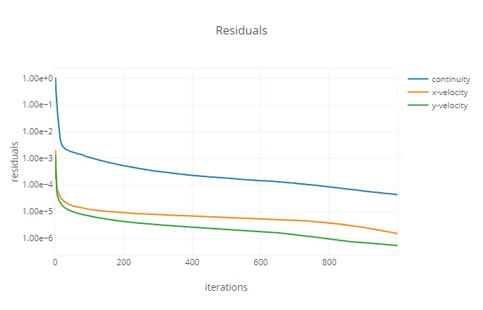
Drag plot :-

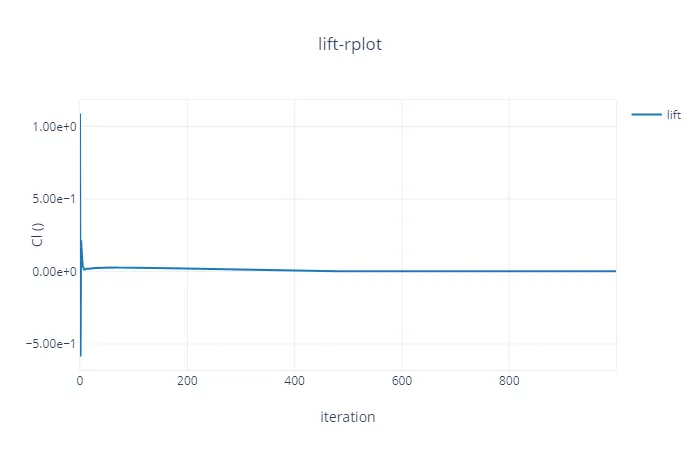
Lift plot :-

Vertex Average Velocity Plot :-

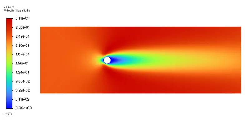
Velocity Cotour :-

Pressure Cotour :-

Vector Velocity Cotour :-

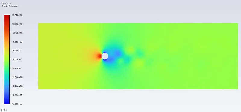
• CASE-2: Re=100, Inlet velocity=2.5, Steady-state solver

Scaled Residuals :-

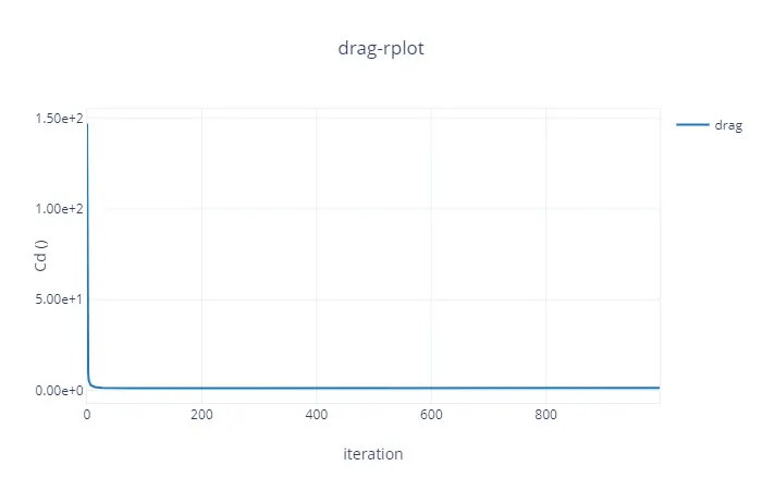
Drag plot :-

Lift plot :-

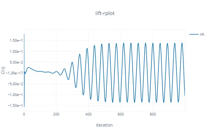
Vertex Average Velocity Plot :-

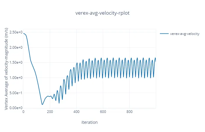
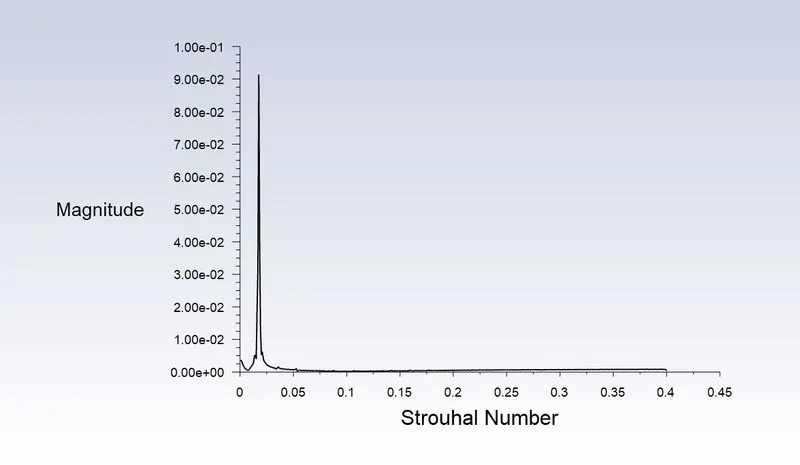
Strohaul Number :-

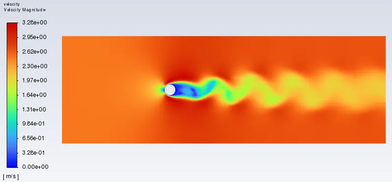
Velocity Cotour :-

Pressure Cotour :-

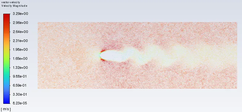
Vector Velocity Cotour :-

Animation :-

https://drive.google.com/file/d/1wn-WcMVrDBkgxEMjfbTZ_zNF2u7WeBl0/view?usp=share_link

• CASE-3: Re=100, Inlet velocity=2.5, Ubsteady-state solver

Scaled Residuals :-

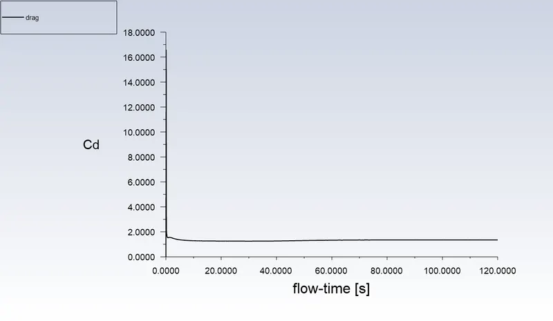
Drag plot :-

Lift plot :-

Vertex Average Velocity Plot :-

Strohaul Number :-

Velocity Cotour :-

Pressure Cotour :-

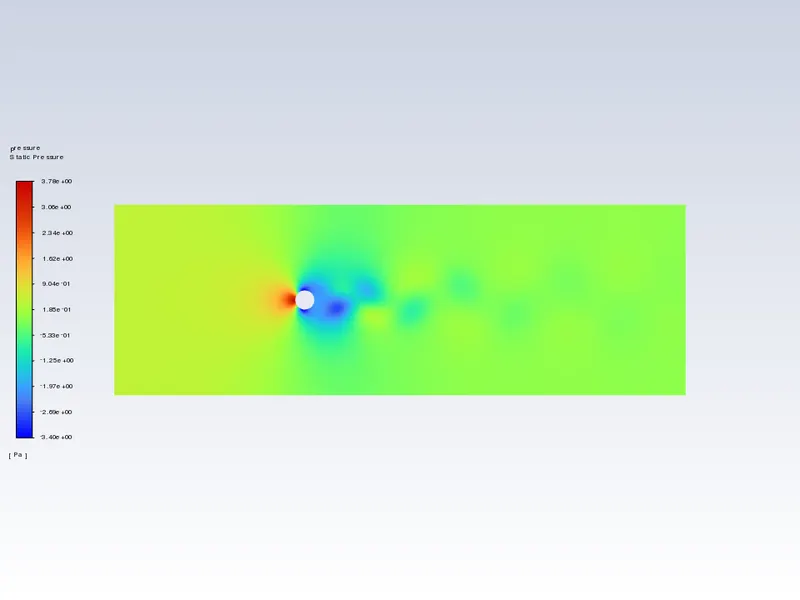
• CASE-4: Re=1000, Inlet velocity=25, Steady-state solver

Scaled Residuals :-

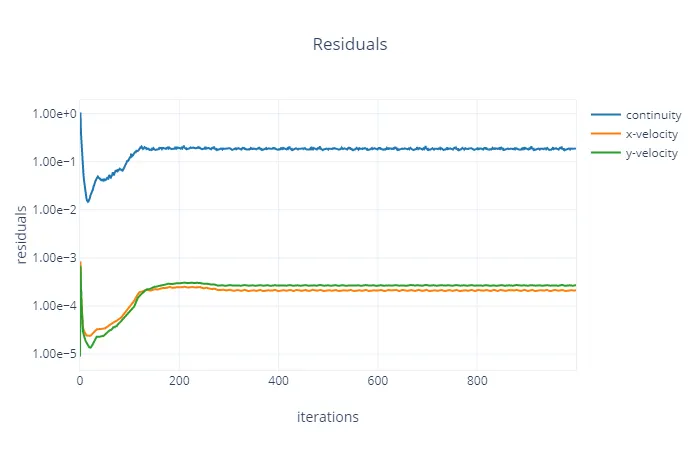
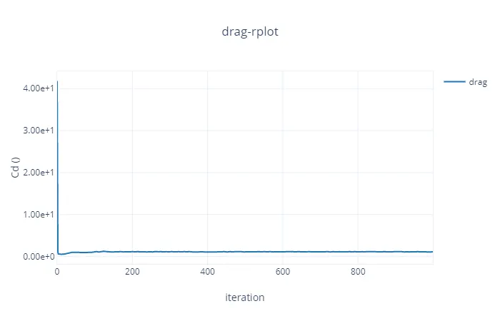
Drag plot :-

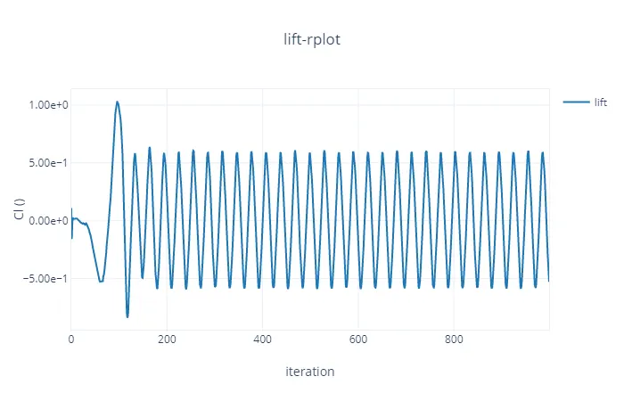
Lift plot :-

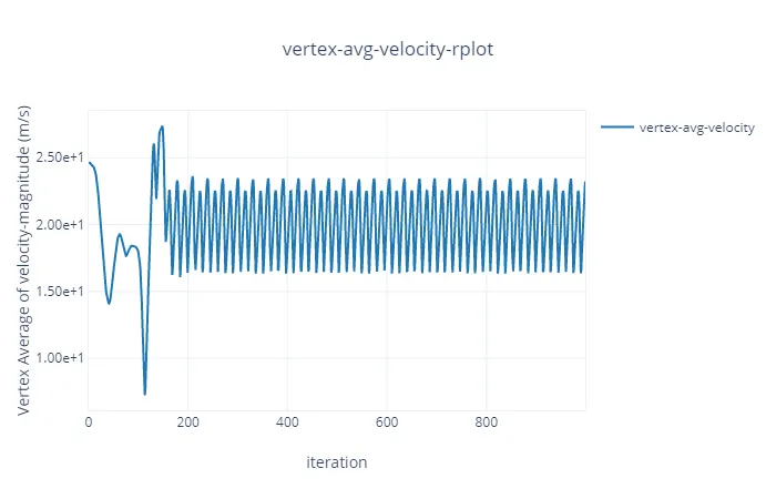
Vertex Average Velocity Plot :-

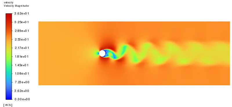
Velocity Cotour :-

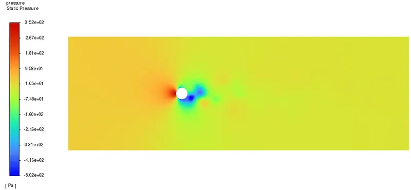
Pressure Cotour :-

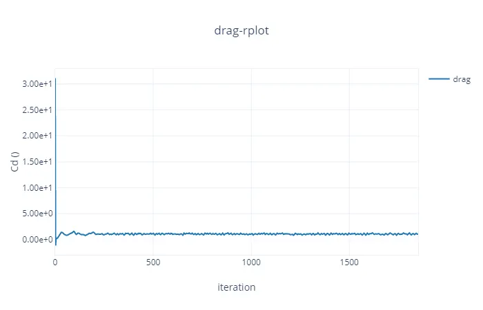
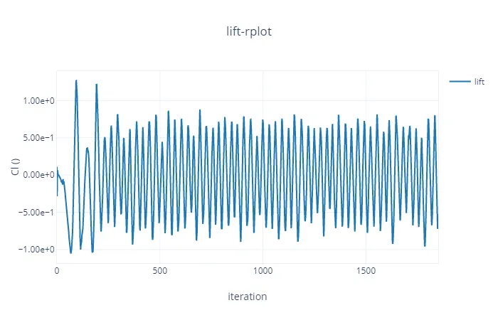
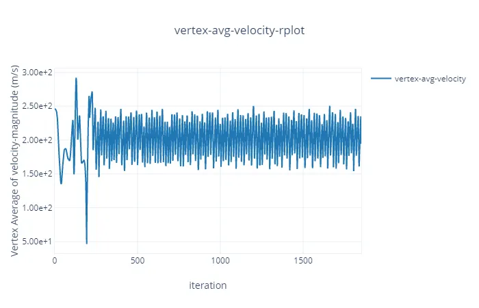
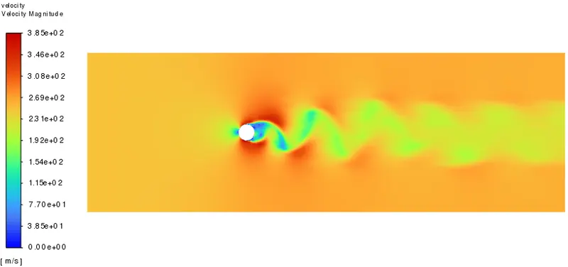
• CASE-5: Re=10000, Inlet velocity=250., Steady-state solver

Scaled Residuals :-

Drag plot :-

Lift plot :-

Vertex Average Velocity Plot :-

Velocity Cotour :-

Pressure Cotour :-

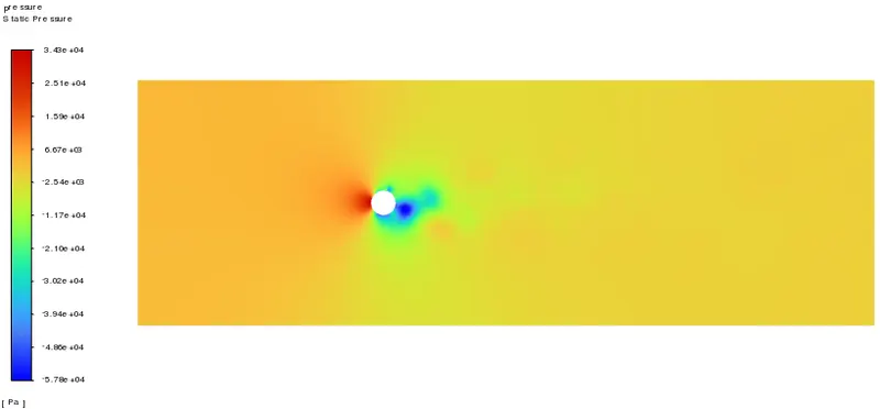
• CASE-6: Re=100000, Inlet velocity=2500, Steady-state solver

Scaled Residuals :-

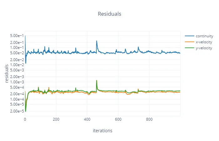
Drag plot :-

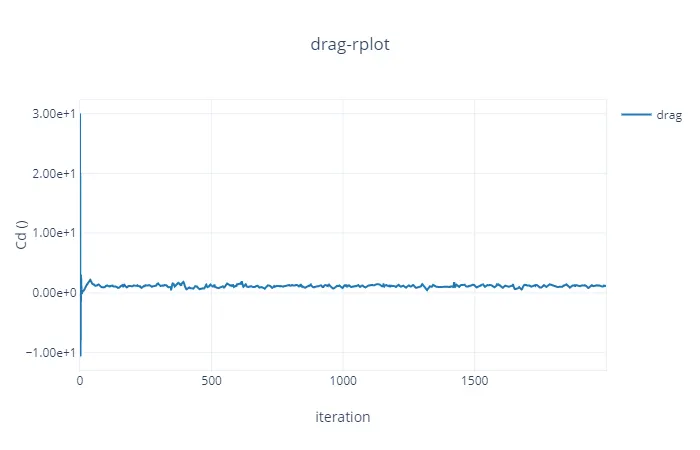
Lift plot :-

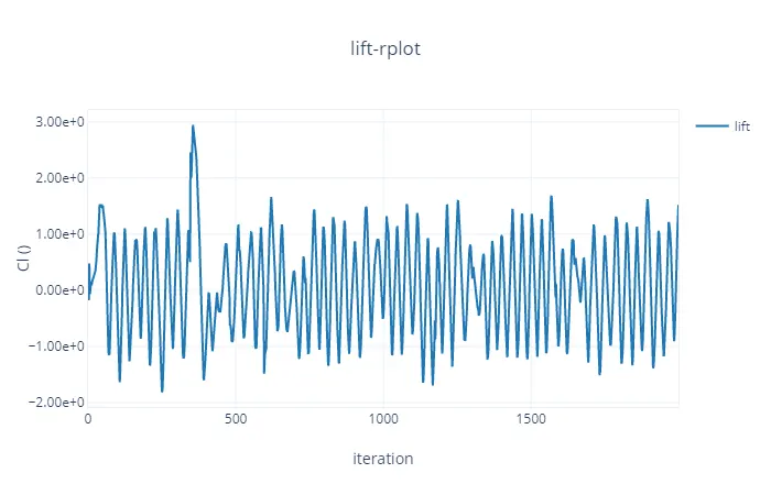
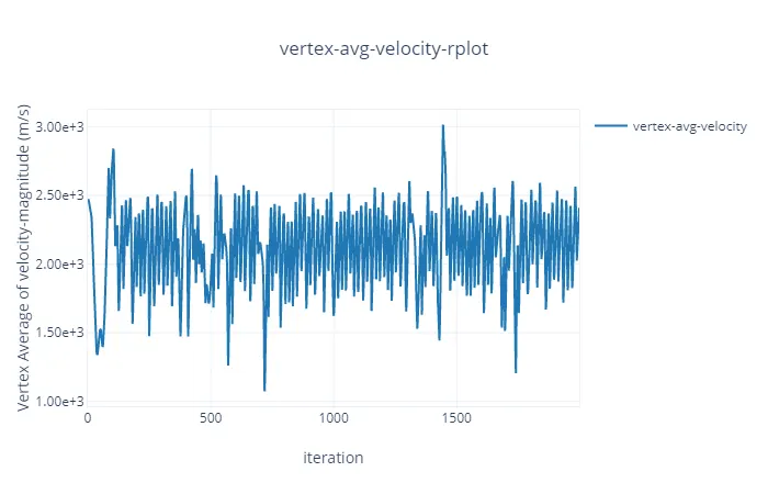
Vertex Average Velocity Plot :-

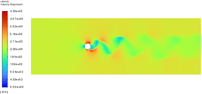
Velocity Cotour :-

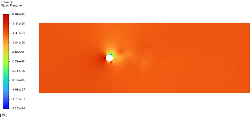
Pressure Cotour :-

Conclusions :-

• Following graph shows the drag efficiency for each case. we can see that it is decreasing as the velocity increases. thishappens as flow separation starts after a certain value of Reynolds number and the viscous drag decreases.
• Following table shows the values of Drag coeff., lift coeff. and vertex average velocity for all the cases.

Cases	Type of flow	Reynolds No. (Re)	Velocity (m/s)	Coeff of Drag (Cd)	Coeff of Lift (Cl)	Vertex-avg.-velocity
1	Steady flow	10	0.25	3.3351935	0.000882	0.105473
2	Steady flow	100	2.5	1.3357814	-0.116760	1.431246
3	Unsteady flow	100	2.5	1.3492274	-0.014649	1.431067
4	Steady flow	1000	25	1.0608328	-0.528028	23.225471
5	Steady flow	10000	250	1.1166724	-0.529470	194.55411
6	Steady flow	100000	2500	1.1771202	1.523061	2408.9072

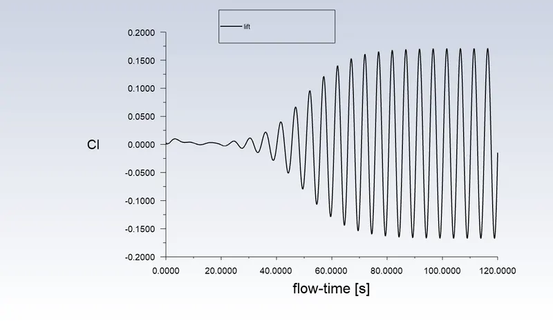
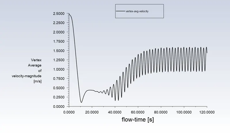
• We can see the fluctuation in the Vertex avg velocity plot that signifies the vortex shedding phenomenon due to which the velocity at the monitor point is oscillating. the phenomenon can also be observed in the Lift plots whose values are fluctuating between positive and negative values due to the oscillations but the average value is 0 due to the shape of the cylinder and no net lift is generated on the body.
• The final iteration values of lift and VAV cannot be used to analyze results like Drag as these values have attained convergence in oscillation. and the last iteration could have stopped at any point from the whole wave.
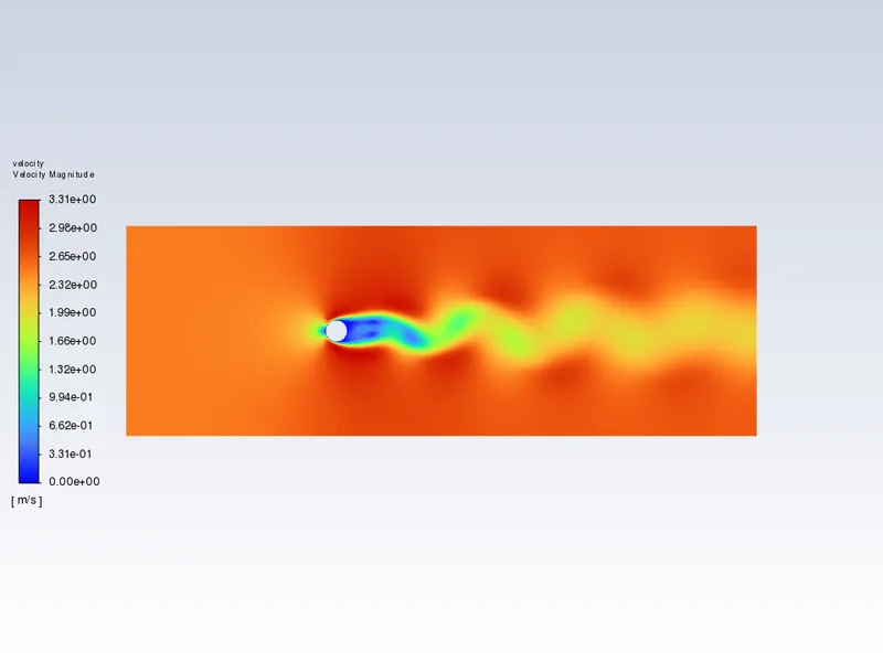
• The animation created for Case 2 shows the vortex shedding and vortices forming behind the cylinder.
• We can also see the flow separation over the surface.
• We can even see that the magnitude of velocity increases on the curve of the cylinder before flow separation.