Week 2 - Flow over a Cylinder.
Objective: To simulate the flow over a cylinder and explain the phenomenon of Karman vortex street
Theory:
When a flow over a cylinder happens at low Reynolds number, let's say at Re=1,the flow is completely attached to the cylinder and the flow adjusts itself such that the flow engulfed the cylinder fully. Here in Reynolds number the characteristic length is given by diameter of the cylinder. The critical Reynolds number for flow over a cylinder is 2x10⁵, at this Reynolds number the flow is laminar over the body of the cylinder. As the Reynolds number increases beyond the critical number the flow is transitioned and becomes turbulent around Re>=2x10⁶.
In the laminar region,the boundary layer is attached to the body at a very low Reynolds number;this type of low Reynolds number flow is called creeping flow.
Now consider the flow over the cylinder at low Reynolds number. At the front of the cylinder on midplane the velocity of the fluid gets converted to pressure energy. At this point the pressure is maximum,this location is called the stagnation point in the flow field. As the Reynolds number is increased ,still being in laminar flow, the flow is attached at the front of the cylinder ,but the boundary layer separates as the flow progresses over the cylinder. Behind the cylinder or above the cylinder i.e at 800 in laminar flow the flow starts to separate. The reason why it separates is explained in the following paragraph.
The pressure is maximum at the front midplane point ,which is called as stagnation pressure. Now the pressure starts to increase as flow starts to traversers uphill of the cylinder , in this time the velocity increases and hence this facilitates the flow in a favorable pressure gradient. Now the pressure is assisting the flow of the fluid around the cylinder. Now the pressure increases for some region and remains constant .This creates an adverse pressure gradient.
In the first half of the cylinder the fluid flows due to pressure difference and in this region there is favorable pressure gradient exists,due to which flow accelerates.In the remaining half of the cylinder now the area increases and pressure is also more downstream. Fluid has its inertia to move in forward direction so the fluid is carried upstream but to increase in flow area the velocity decreases and pressure force increases. This increase in pressure forces causes unfavorable or adverse pressure gradient and fluid retards,But the fluid coming from downstream pushes the retarding fluid and due to this there are vortex formation happening. At a low Reynolds number this phenomenon is very dominant. Behind the cylinder where vortex formation takes place , this region is called the wake region. The vortices formed are periodic in nature and have some frequency of their own. These types of swirling vortex are called von Karman vortex streets. The vortex formed to gain energy from the flowing fluid and dissipate it in the flow field after some distance with the help of viscosity.
In the wake region pressure drops and is much less than the stagnation pressure at the front ,due to this there is pressure force imbalance which causes drag.
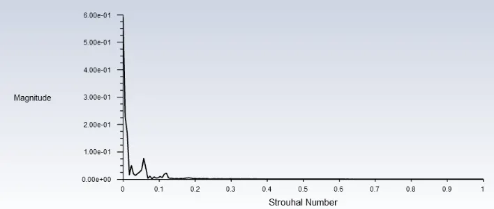
Part A:Simulating the flow over the cylinder with steady and transient and calculate the Strouhal Number.
Step 1:
Generate the geometry over which simulation is to be carried out. The geometry is prepared in spaceclaim.The dimensions of the geometry are given below. The diameter of the cylinder is 2 m. This is external flow so an enclosure is to be made to simulate the external flow. This enclosure is to be made in such a way that the effect of the boundary layer formed on the body should not be felt on the walls of the enclosure.
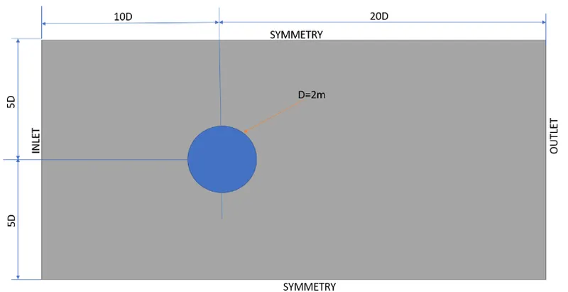
Note the plane in which the sketch is drawn.Here we have taken the XY plane ,so while computing drag and lift the force vector will be in negative x and positive y direction respectively.After creating the sketch convert the sketch to surface by using pull command.We will get a surface as shown below.
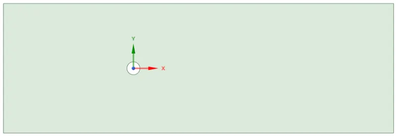
Step 2: Meshing
After opening the Ansys Mesh use the default settings for meshing and generate the mesh. We will get a quadrilateral dominant mesh as shown below.
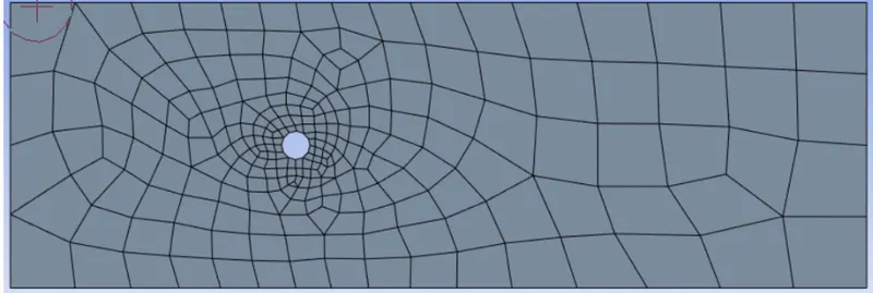
Now to make the mesh proper and fine we need to use different settings. First is we need to convert the mesh into triangular dominant mesh. Therefore right click on the mesh and select insert then select methods.
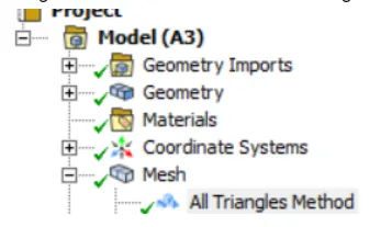
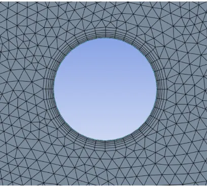
After selecting the methods select the triangle as methods and then update the mesh.After this again right click on the mesh and select sizing from methods. Here select the edge filter and select the edges of the cylinder wall.In the details select the number of divisions in type and provide 36 divisions.This is just to make the edge of the wall smooth so that the effects near to the wall are captured accurately.Update the mesh. Now near the wall boundary layer will be formed to capture this we need to refine the mesh near the wall. This is done by inserting the method ‘inflation’. In this provide the number of layers 6 the growth rate of each layer is 20% by default.
Now update the mesh and give the size of each cell as around 0.2m.You will get the below mesh.
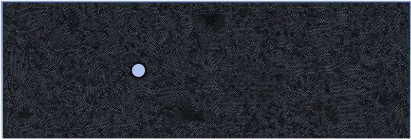
Now we need to provide the name for boundary condition, inlet, outlet,symmetry,wall.
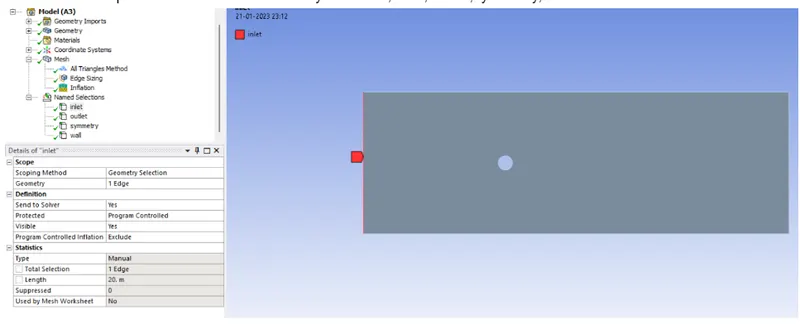
Close the meshing workbench and update the ansys workbench. This same mesh is used for all simulations.
Step 3: Setup/Pre-processing
Open Fluent,the mesh will load up.Now add a custom material with density as 1 kg/m3 and dynamic viscosity as 0.02kg/ms.
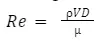
Here Re is to be kept at 100 as per the question. D=2m,=0.02 kg/ms,So the velocity over here comes out be 1 m/s
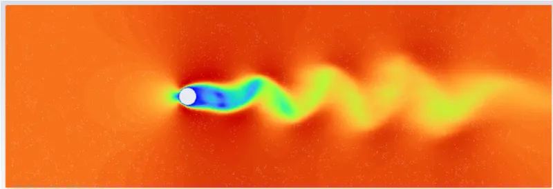
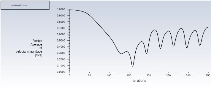
Apply boundary conditions. Make sure you have selected the steady state simulation and model for the simulation problem as laminar. Now add monitor point by creating it in the results tab at a location of 4D,i.e;8m.Again come back to the solution tab select the definition - surface report - vertex average. Select the monitor point which was created earlier. At this point we will get to see how velocity is fluctuating. Select hybrid initialization and then select methods and select SIMPLE method. It stands for SEMI IMPLICIT METHODS FOR PRESSURE LINKED EQUATIONS.Now provide the number of iterations as 350 and run the calculation. After the calculations are completed you will get the following plots and contours.
Velocity contour:
Vertex average of velocity magnitude plot:
Strouhal Number:
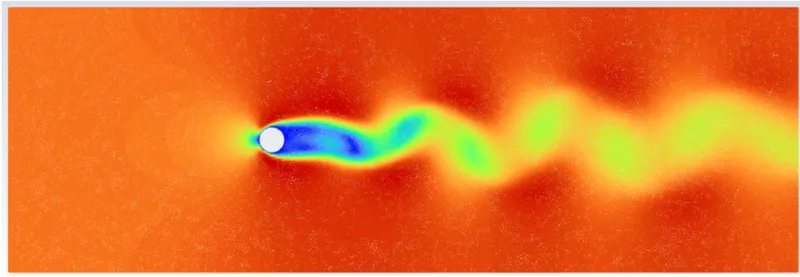
Similar steps are to be followed for transient simulation,we just need to switch on the transient simulation and while performing the simulation we need to enter the number of time steps as 800 and time step size as 0.1s.
Velocity contour:
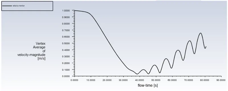
Vertex average of velocity magnitude plot:
Strouhal Number
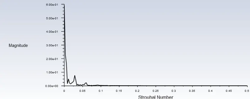
In steady simulation we get to see the vortex generated and the frequency of the fluctuation of the velocity is also steady, this can be seen from velocity vertex average plot.On the other hand in transient simulation the velocity fluctuations goes on increasing. The vortex can be captured both in steady and transient but transient simulation gives a realistic picture.
Part B: Calculate the coefficient of drag and lift over a cylinder for Reynolds number 10,100,1000,10000 with steady state solver.
Same geometry and mesh settings are used for this part. Here the only thing which is changing is inlet boundary condition, For each Reynolds number velocity is calculated as above. All the simulations are to be done using steady state solver.
Re=10
Inlet velocity=0.1m/s
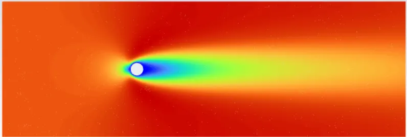
Velocity contour:
Velocity plot vertex average:
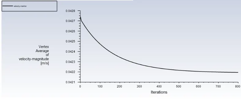
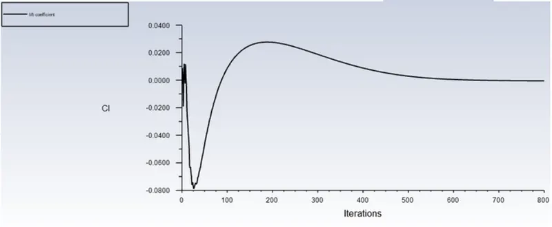
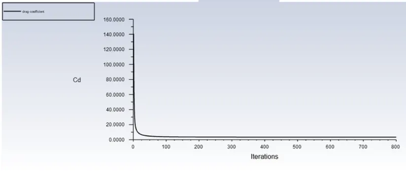
For Reynold number 10,the flow is creeping in nature.We can see that there is no vortex shedding happening as expected. Also the velocity goes on decreasing as time progresses and becomes constant.This can be see from the plot. The drag at this Reynolds number is very much low
Lift plot:
Drag plot:
Re=100
Inlet velocity=1m/s
For Re=100, the von Karman vortex can be seen.This is because as the velocity increases the flow separation occurs and vortex formation starts.
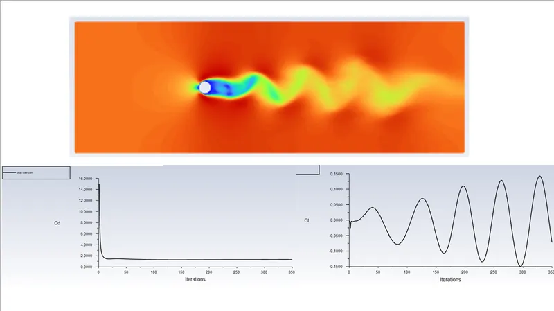
We can see that drag coefficient also increases and there is variation in lift coefficient value. As Re goes on increases we can see the intensity of vortex also increase and they became some what turbulent and have higher frequency.
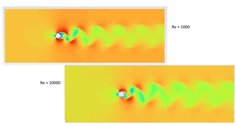
As Re is increased the vortex generated become more chaotic and hence drag on the cyllinder is also increased tremendously.