Week 2 - Flow over a Cylinder.
Week 2 - Flow over a Cylinder.
Aim:
To Simulate the flow over a cylinder and explain the phenomenon of Kármán vortex street. We shall simulate and study in two parts as follows,
PART-I
- To Simulatethe flow with the steady and unsteady case and calculate the Strouhal Number for Re= 100.
PART-II
- To Calculate the coefficient of drag and lift over a cylinder by setting the Reynolds number to 10,100,1000,10000 & 100000. (Run with steady solver)
- To Discuss the effect of Reynolds number on the coefficient of drag.
Introduction:
To start with the simulation topic - Simulation of flow over a circular cylinder and discussion on Karmen Vortex street formation. Here, two broad concepts is discussed which looks very basic but has a wide application regarding the physics behind them.
Flow over a circular cylinder: Cylinder is a blunt body, meaning it doesn’t have a leading edge or a trailing edge like an airfoil. Also, cylinder is a basic cross-sectional reference for all kinds of blunt bodies e.g., flat plates, square rod, airfoil be it positive or negative lift.
This flow over a cylinder can be related to a flow over a tree or a chimney for different Reynolds number, for e.g,.flow over a tree during a normal windy day and during a hurricane has an effect on the tree as well as the fluid flowing over it.
During initial days of development of aerodynamics, Bernoulli studied concepts of lift with a circular cylinder. Hence circular bodies are a great start to study fluid flow concepts.
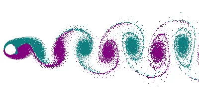
Karmen Vortex street: It is a phenomenon of vortex formation and shedding at various velocities (usually denoted in Reynolds number). This vortex formation happens when an object moves in a stationary fluid or vice versa. Let us see Karmen vortex street phenomena briefly in the following.
Theory of the topic and its importance in practical applications:
In fluid dynamics, a Kármán vortex street (or a von Kármán vortex street) is a repeating pattern of swirling vortices, caused by a process known as vortex shedding, which is responsible for the unsteady separation of flow of a fluid around blunt bodies.
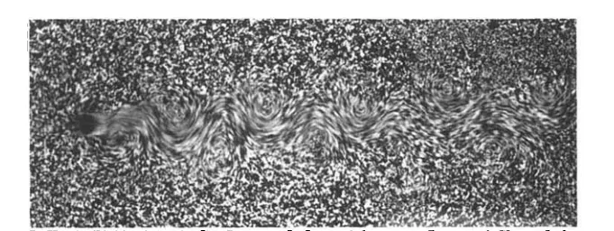
A vortex street will form only at a certain range of flow velocities, specified by a range of Reynolds numbers (Re), typically above a limiting Re value of about 90. The Reynolds number for a flow is a measure of the ratio of inertial to viscous forces in the flow of a fluid around a body or in a channel, and may be defined as a non-dimensional parameter of the global speed of the whole fluid flow, Reynolds number is given by
Re = ρVL / μ
Where, ρ is the density of the fluid.
V is the free stream velocity
L is the Length or hydraulic diameter
μ is the absolute viscosity of the fluid.
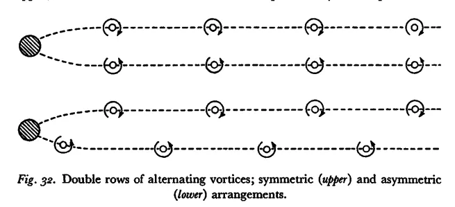
Vortex formation doesn’t occur at lower Reynolds number, when the Reynolds number increases the vortex formation starts proportionally with increasing Reynolds number. When the Reynolds number is sufficiently higher, Karman Vortex shedding occurs. This shedding can be symmetric at transition regimes and asymmetric at turbulent regimes. This vortex shedding oscillates periodically leading to a singing like occurrence, this is given mathematically by Strohaul number
St = fL / U
Where, f is frequency of vortex shedding
L is characteristic length or the hydraulic diameter
U is flow velocity.
Practical applications:
As said earlier, this topic finds a wide variety of applications in a variety of industries. A few of them are illustrated below.
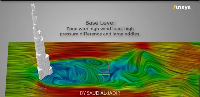
Von Karmen vortex street phenomena is extensively used in skyscraper designs to reduce the drag and wake region behind the buildings so as to avoid oscillation of the building to the upcoming wind. World’s tallest building Burj Khalifa is designed and constructed with this concept.
Wing tip vortices are formed at the tip of wings in airplanes and fighter jets, this is overcome by a small projection at the tip to avoid formation of vortices near to the wing tip.

Karman vortex street over a light pole makes it to oscillate in a certain frequency, this oscillation can lead to fatigue failure of the pole. This can be studied in advance and providing reinforcements can overcome this problem.

Solving and Modeling approach:
We shall solve the case in two parts as discussed in Aim.We will be using ANSYS Fluent solver to create the geometry and perform unstructured tria CFD mesh with boundary definitions, setup the physics of fluid flow and run the iterations to get solutions, using post processing to interpret the data in form of plots,contours, vectors etc.,
For Re 100 we shall perform steady and transient study flow using RANS method. For other cases such as Re 10 to 100000 we shall perform steady state flow study. Then, we tabulate the case study results and compare it with the open literature or book data results to validate the simulation.
Preprocessing and Solver setting:
Let us open ANSYS workbench, now opening Fluent flow can be done by drag and drop in the schematic window or by double clicking on Fluent. The fluent workflow is in a series of steps such as GEOMETRY > MESH > SETUP > SOLUTION > RESULTS. Each step has to be completed for the next step to initialize.
Part 1:
Let us discuss in detail;
GEOMETRY >
In the Fluent, right click on the Geometry and select New SpaceClaim Geometry. The space claim application opens, select FILE > NEW and we can create a geometry. Use SKETCH and make a sketch as follows.
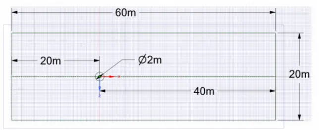
We can use PULL tool to make a plane from this sketch, or we can use RETURN TO 3D mode to do the same.
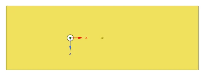
We are good to go now. Once the geometry is ready, we can close space claim and check that the fluid flow (fluent) geometry is updated indicated by a green tick.
MESH >
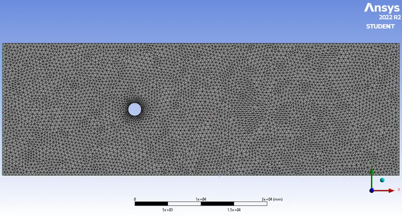
Right clicking on the Mesh and selecting edit opens the Mesh window. Mesh window is preloaded with the geometry we have worked on earlier, so clicking on the GENERATE MESH should create a mesh automatically. The default mesh is mixed mesh here, but we are interested in tria type mesh. So, right clicking on the mesh and going to INSERT > METHOD > ALL TRIANGLES. We shall add inflation layers with 0.5 as first layer thickness and add 6 layers. The desired mesh size we can use is 500 mm. We shall create a monitoring point at 8m from the cylinder in the wake region. In this monitoring point we shall study the average velocity. Any changes made, click on the update icon to update the mesh details or else there is an indication of a thunderbolt sign asking the user to update.
We shall name the entry and exit surfaces such as Inlet, Outlet, Wall by selecting the respective faces and using the ‘N’ button and name them as symmetry. Once this is done, we should see a green tick near Mesh. we can close the mesh window.
SETUP >
Right clicking on the Setup, opens the Fluent launcher. In the Fluent launcher select 3D, Double precision and select the number of cores as per the user system configuration and click on start.
Upon opening, there are some selections to be done to define the simulation definitions, we shall select Type: Pressure based, Velocity Formulation: Absolute, Time: Steady. Under the Physics tab, we can turn on viscous and select laminar.
Under the materials we shall select air as our default material with material type as fluid. We can create a copy of the material and change the density to 1 Kg/m^3 and viscosity to 0.05 Kg/m-s
Under the cell zone conditions, select the volume and it should show type as fluid by default.
We can proceed to define boundary conditions, as follows
Inlet X : velocity magnitude = 2.5 m/s (For Re 100)
Outlet should be a pressure outlet.
upper and lower walls can be set as symmetry.
For generating reports, click on the Solution > Reports > Definitions > New > Force Report > Drag coefficient for the drag coefficient over the cylinder wall. Similarly we can make a report for lift coefficient, and for Vertex average velocity we can use Solution > Reports > Definitions > New > Vertex average > Velocity. We shall input compute from INLET in reference values and in the initialization as well. Now, it's time to start the simulation. In order to start the simulation for the above set up physics, we need to initialize the entire flow field by clicking on the t=0 initialize icon. In the Run Calculation we can input the number of iterations to be run (in this case 350) and clicking on the Calculate should start the iterations. After iterations, we get scaled residuals, average temperature plot and standard deviation plots.
We need velocity and pressure contours as well, to get them we can create a transverse cut plane i.e, XY plane and make new contour in Results > Graphics > Contours > New pressure for pressure contour and velocity for velocity contour. The scale can be edited by double clicking on it.
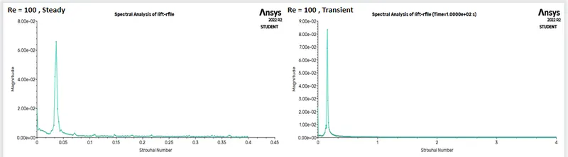
Strouhal number plot also can be plotted using FFT plot in the results tab. The strouhal data can be exported to an excel file to find out the maximum strouhal number.
In the Outline view under Simulation Reports, clicking on the Report Outline > Generate should generate a Ansys Fluent Simulation Report which is automatically generated with all the information of the simulation in it. This can be exported as a PDF also. We are done with setup, we can close the setup.
SOLUTION >
Since some solution is calculated in the setup itself, we can see the green ticks in both setup and solution too.
RESULTS >
Right clicking on the Results should open the Post processor. Default view is a wireframe model, we can turn on the symmetry 1 to view contours and vectors. Selecting the Vector and selecting the symmetry 1 plane creates a velocity vector.
Similar to setup and solution, all contours and plots can be created here, in addition to that we can create an animation of the velocity contour by clicking on AUTOSAVE during the solution and clicking on ANIMATE select make movie and save in desired location.
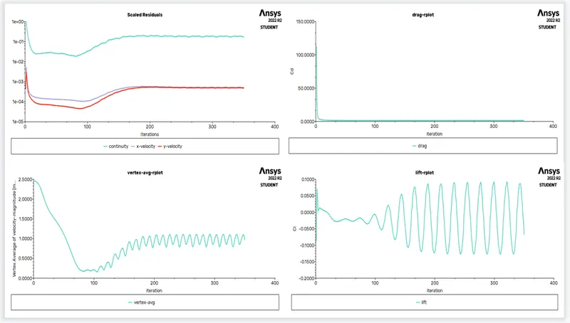
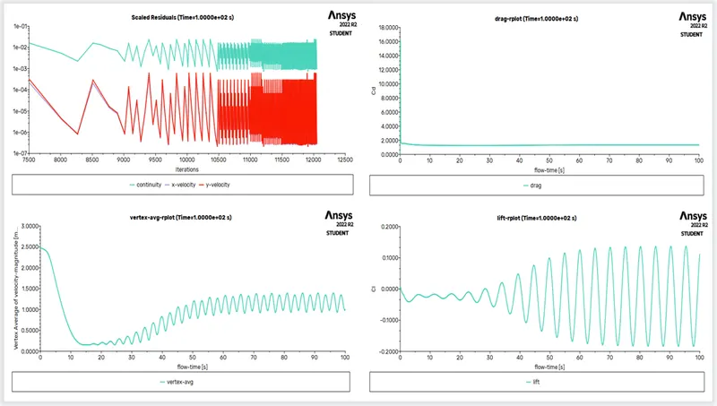
For Case 2 (Re 100, Transient), we can simply Duplicate the existing Case 1 Fluent file. Change the type to TRANSIENT in the Setup and add time step size as 0.01 and no. of time step as 1000 and run the simulation and gather data like we did with case 1.
Similarly, we can follow the above procedure for the other cases from Re 10 to Re 100000, using steady flow in fluent solver. with velocities as 0.25 m/s for Re 10 upto 2500 m/s for Re 100000, with multiplication factor of 10 for each Reynolds number respectively.
RESULTS:
After repeating the similar manner of simulation procedures for all 2 parts from aim, we have a handful of data to compare and study. We shall put in order all the contours, plots and vectors for us to compare and come to a conclusion. Here, only the results of all cases are displayed, its inference and interpretation shall be discussed briefly in conclusion.
Part 1:
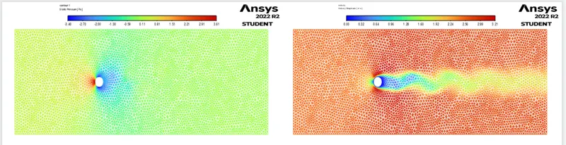
Re = 100 , Steady state
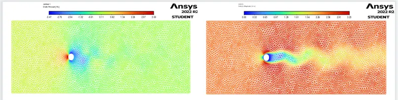
Re = 100 , Transient state
Strouhal number plot
Part 2:
For Re 10 to 100000,
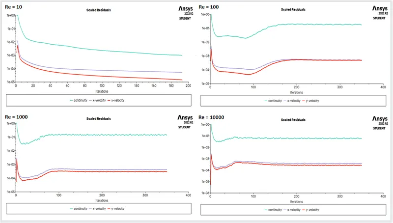
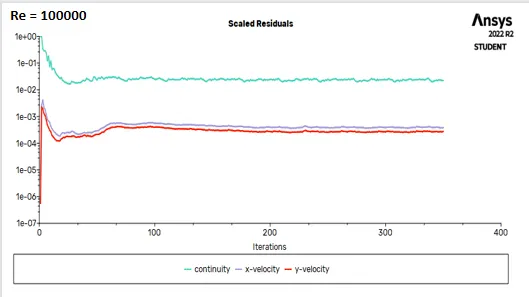
Scaled Residuals
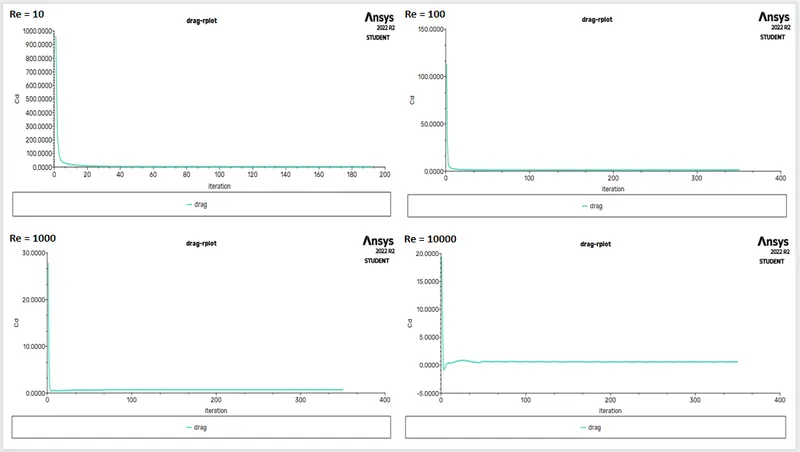
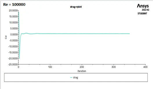
Drag plots
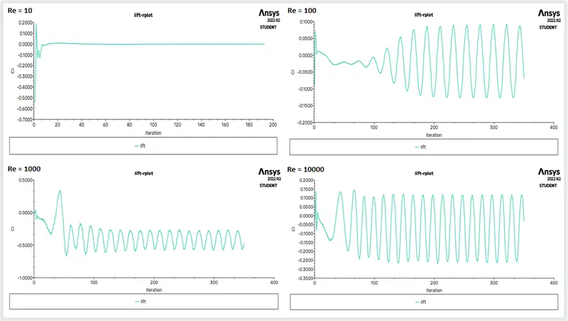
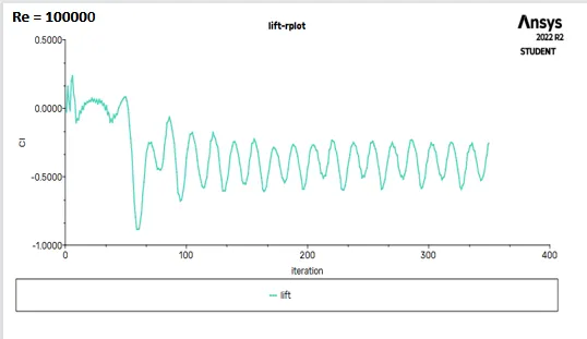
Lift Plots
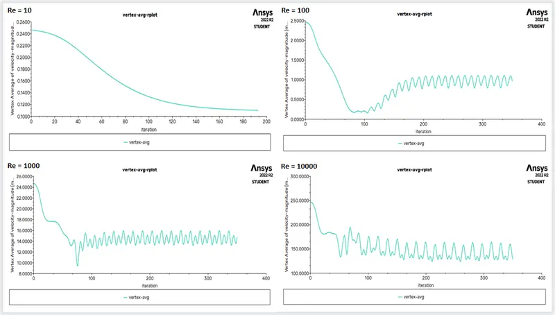
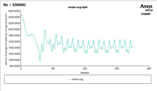
Vertex average Velocity plots
Pressure Contours
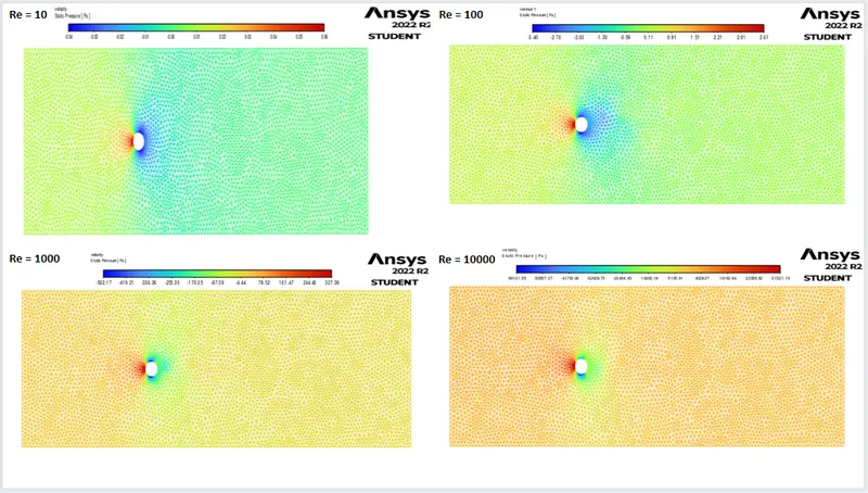
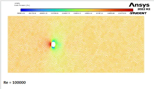
Velocity Contours
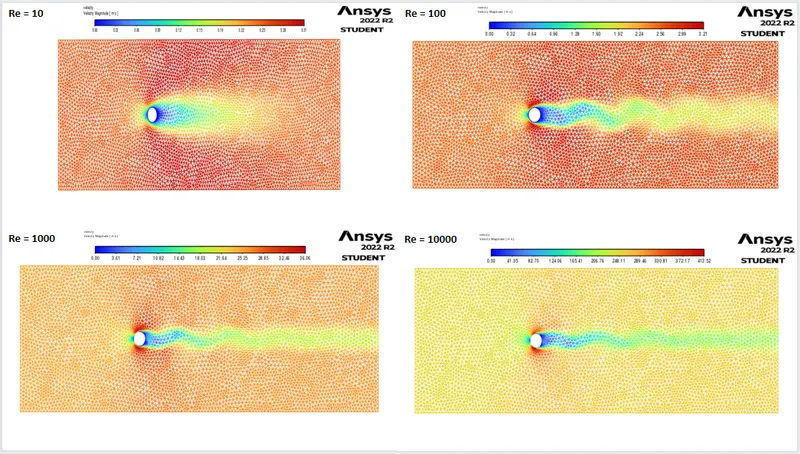
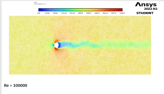
Animation of Velocity contour for Re = 10000
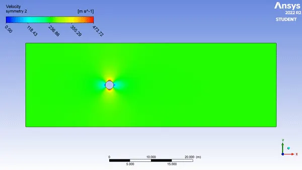
Conclusion:
The compilated results in the tabulated form are as follows for both part 1 and part 2,
| Re | Cd | Cl | Vertex average Velocity(m/s) |
| 10 | 3.331 | -0.0006 | 0.110 |
| 100 | 1.332 | -0.0671 | 0.969 |
| 1000 | 0.716 | -0.0285 | 14.738 |
| 10000 | 0.615 | -0.4666 | 128.76 |
| 100000 | 0.569 | -0.2491 | 1429.59 |
Theoretical comparison of Cd
| Reynolds no | Theoretical Cd | Numerical Cd | error |
| 10 | 3.5 | 3.331 | 4.82% |
| 100 | 1.4 | 1.332 | 4.85% |
So error computable is less than 5%
INFERENCES:
Here, from the steady and transient study for Re 100 we can see that the results are almost similar. The strouhal numbers are also similar for steady state 0.065 and for transient state 0.083. Also, from Re and Cd comparison table as the Reynolds number increases coefficient of drag decreases while the coefficient of lift increases.
The solution is converged for lower Reynolds number whereas the solution for other higher Reynolds number can be considered as converged from the graphs.
since the object is fixed and the lift coefficient increases with increase in Reynolds number, the oscillations occur in the vortices. The same can be confirmed with the velocity contours comparison as well.
References:
https://www.sciencedirect.com/science/article/pii/S0307904X08000243
Aerodynamics : selected topics in the light of their historical development by Theodore von Karman.