Week 2 - Flow over a Cylinder.
CHALLENGE - 2: Flow Over a Cylinder
AIM:
To perform the simulation of flow over a cylinder by using ANSYS FLUENT for the given cases.
OBJECTIVE:
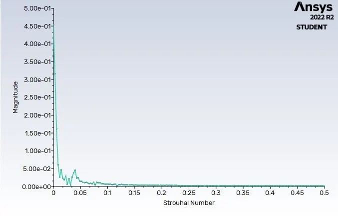
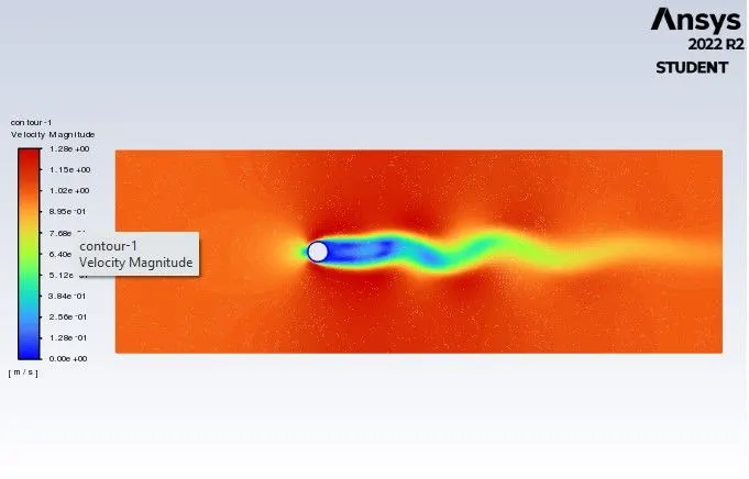
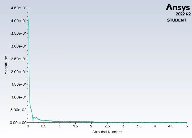
- To simulate the flow over a cylinder with the steady and unsteady case and calculate the Strouhal Number for Re= 100.
- To calculate the coefficient of drag and lift over a cylinder by setting the Reynolds number to 10,100,1000,10000 & 100000.
- To discuss the effect of Reynolds number on the coefficient of drag.
- To plot of the coefficient of drag and lift for different cases and to plot the contour of vortex shedding behind the cylinder.
PROCEDURE:
1. Open ANSYS Workbench 2022R2 select Fluid Flow (Fluent) from Toolbox.
2. Rename the file and left click Geometry and select New Spaceclaim Geometry.
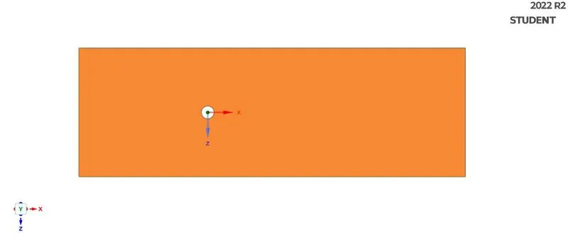
3. Create the geometry as shown below using rectangle tool and construction line tool. The circle shown represents the cylinder and its diameter is considered as 2m. From the centre of circle to ithe distance to inlet and outlet are 20m and 40m respectively. The length of inlet and outlet are 20m. After creating the geometry select the face and create the surface to the geometry.
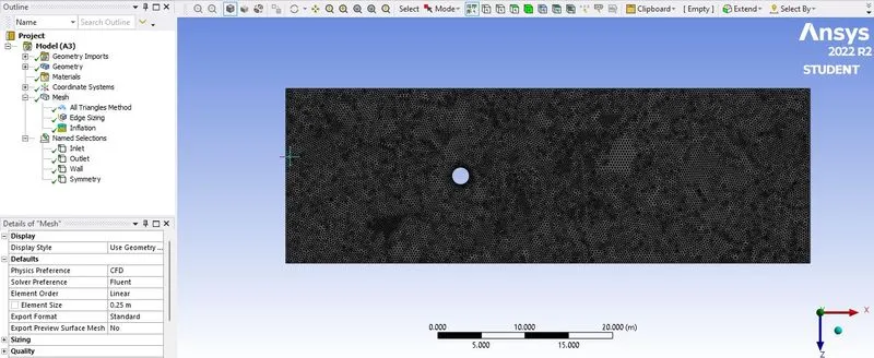
5. Close SpaceClaim and double click on Mesh. Meshing window will appear. Mark Inlet, Outlet, Symmetry and Walls on geometry by right clicking each part and selecting Create Name Selection. Now select the mesh from the tree and generate mesh with an appropriate element size. From insert opstion select sizing and provide number of divisions to the circular part. Similary select method and provide triangular meshing by selecting the whole body. Also provide the inflation layer to the circular part. Inflation layer helps to create uniform meshing on the surface where it needed The figure shown below show the geometry after meshing.
Note: More refined mesh would provide an accurate simulation but it take more computational time. Since the problem is solved using student version of ANSYS there is limitation in number of mesh elements.
6. Close Meshing and double click on Setup, select Double Precision and Fluent window will open. Check all the values and make necessary correction if needed.
7. Select appropriate conditions mentioned below.
PART-1
Case 1: Steady case with Re = 100
Time - Steady
Viscous - Laminar
Material - User defined with Density = 1(kg/m3) and viscosity = 0.02(kg/(ms))
Cell Zone Conditions
Volume - Fluid - Used defined
Boundary Conditions
Inlet - Velocity Inlet, Velocity = 1m/s.
Wall - Wall
Outlet - Pressure Outlet
Symmetry - Symmetry
Solution Initialization - Hybrid Initialization.
Case 2: Unsteady case with Re = 100
Time - Transient
Viscous - Laminar
Material - User defined with Density = 1(kg/m3) and viscosity = 0.02(kg/(ms))
Cell Zone Conditions
Volume - Fluid - Used defined
Boundary Conditions
Inlet - Velocity Inlet, Velocity = 1m/s.
Wall - Wall
Outlet - Pressure Outlet
Symmetry - Symmetry
Solution Initialization - Hybrid Initialization.
PART-2
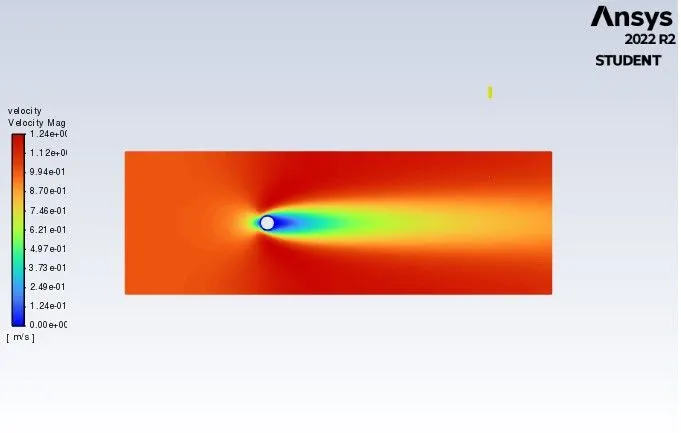
Case 1: Steady case with Re = 10
Time - Steady
Viscous - Laminar
Material - User defined with Density = 1(kg/m3) and viscosity = 0.2(kg/(ms))
Cell Zone Conditions
Volume - Fluid - Used defined
Boundary Conditions
Inlet - Velocity Inlet, Velocity = 1m/s.
Wall - Wall
Outlet - Pressure Outlet
Symmetry - Symmetry
Solution Initialization - Hybrid Initialization.
Case 2: Steady case with Re = 100
Time - Steady
Viscous - Laminar
Material - User defined with Density = 1(kg/m3) and viscosity = 0.02(kg/(ms))
Cell Zone Conditions
Volume - Fluid - Used defined
Boundary Conditions
Inlet - Velocity Inlet, Velocity = 1m/s.
Wall - Wall
Outlet - Pressure Outlet
Symmetry - Symmetry
Solution Initialization - Hybrid Initialization.
Case 3: Steady case with Re = 1000
Time - Steady
Viscous - Laminar
Material - User defined with Density = 1(kg/m3) and viscosity = 0.002(kg/(ms))
Cell Zone Conditions
Volume - Fluid - Used defined
Boundary Conditions
Inlet - Velocity Inlet, Velocity = 1m/s.
Wall - Wall
Outlet - Pressure Outlet
Symmetry - Symmetry
Solution Initialization - Hybrid Initialization.
Case 4: Steady case with Re = 10000
Time - Steady
Viscous - Laminar
Material - User defined with Density = 1(kg/m3) and viscosity = 0.0002(kg/(ms))
Cell Zone Conditions
Volume - Fluid - Used defined
Boundary Conditions
Inlet - Velocity Inlet, Velocity = 1m/s.
Wall - Wall
Outlet - Pressure Outlet
Symmetry - Symmetry
Solution Initialization - Hybrid Initialization.
Case 5: Steady case with Re = 100000
Time - Steady
Viscous - Laminar
Material - User defined with Density = 1(kg/m3) and viscosity = 0.00002(kg/(ms))
Cell Zone Conditions
Volume - Fluid - Used defined
Boundary Conditions
Inlet - Velocity Inlet, Velocity = 1m/s.
Wall - Wall
Outlet - Pressure Outlet
Symmetry - Symmetry
Solution Initialization - Hybrid Initialization.
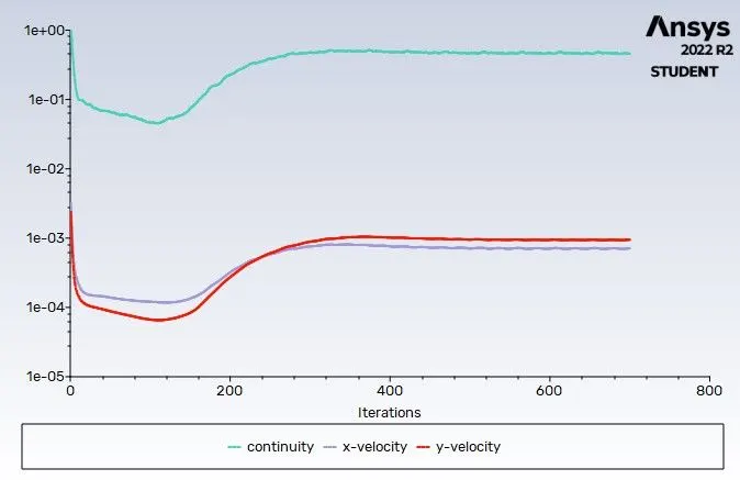
8. After assigning all the factors click on Run Calculation and set number of iteration for steady case and for transient case set number of time steps and calculate. The figure below shoews the residual plot after calculation for case 1 from part 1.
9. Repeat these steps for all the cases and compare the results.
RESULTS AND DISCUSSION:
PART-1
Case 1: Steady case with Re = 100
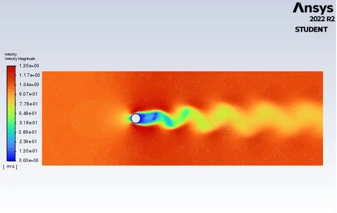
a. Velocity Contour
b. Strouhal Number
Case 2: Unsteady case with Re = 100
a. Velocity Contour
b. Strouhal Number
Note: Animation files for both case 1 and 2 are mentioned in the below link.
PART-2
Case 1: Steady case with Re = 10
a. Velocity Contour
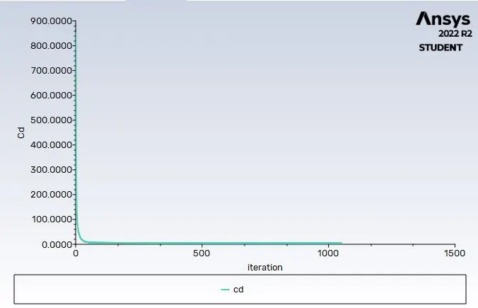
b. Coefficient of Drag
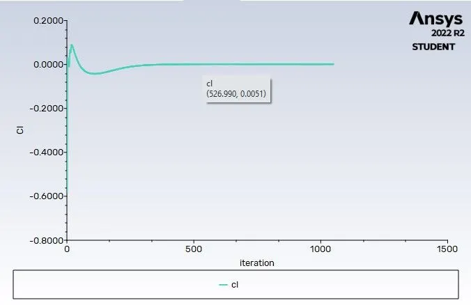
c. Coefficient of Lift
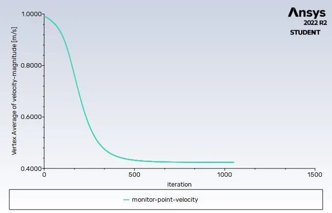
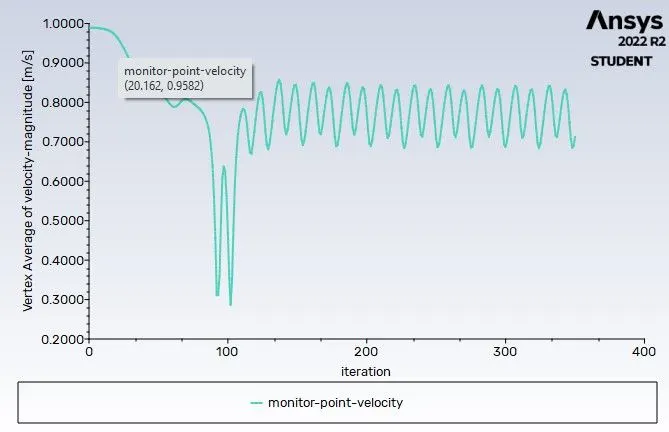
d. Vertex average velocity at monitor point
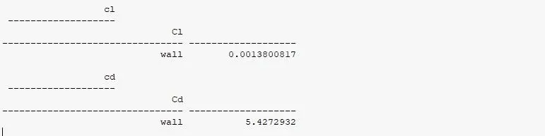
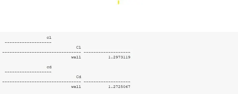
e. Computed values of Coeff. of drag and Coeff. of lift
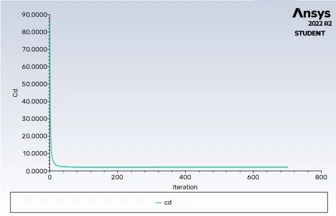
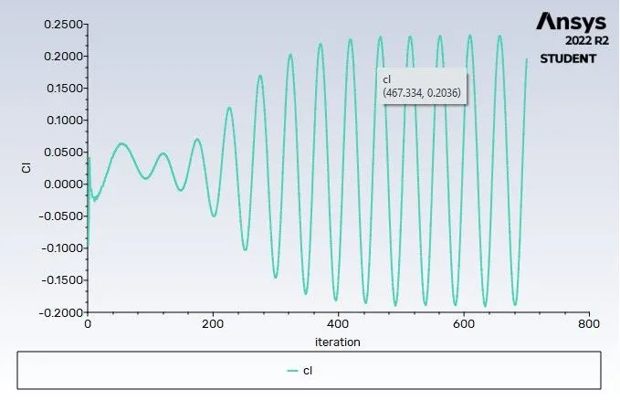
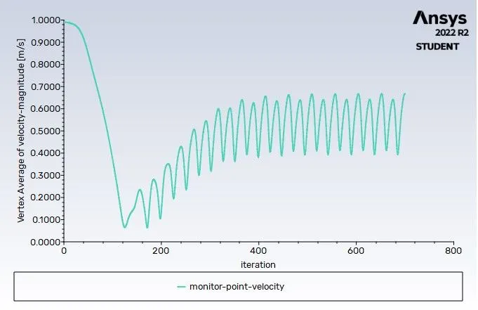
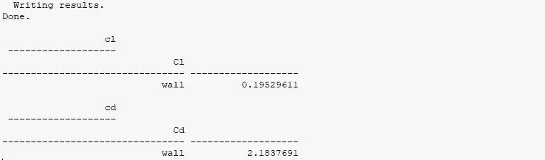
Case 2: Steady case with Re = 100
a. Velocity Contour
b. Coefficient of Drag
c. Coefficient of Lift
d. Vertex average velocity at monitor point
e. Computed values of Coeff. of drag and Coeff. of lift
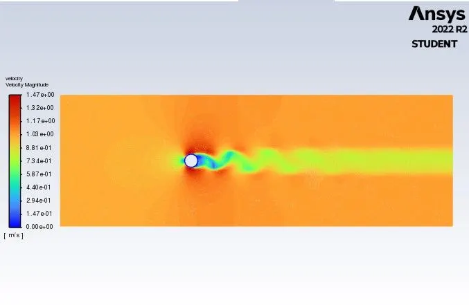
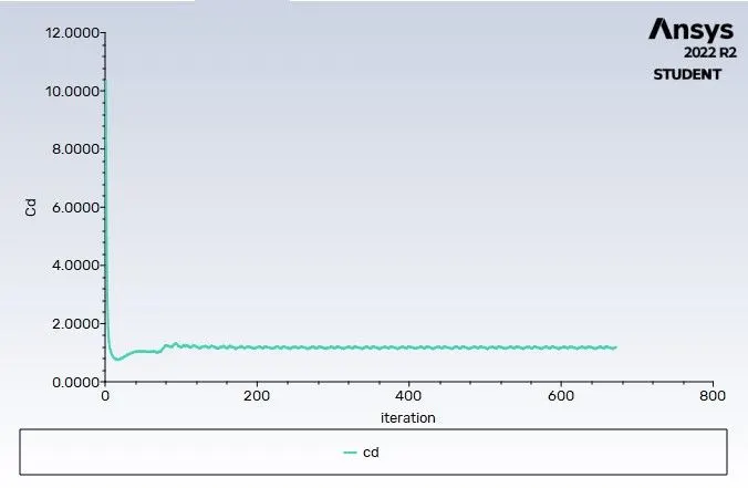
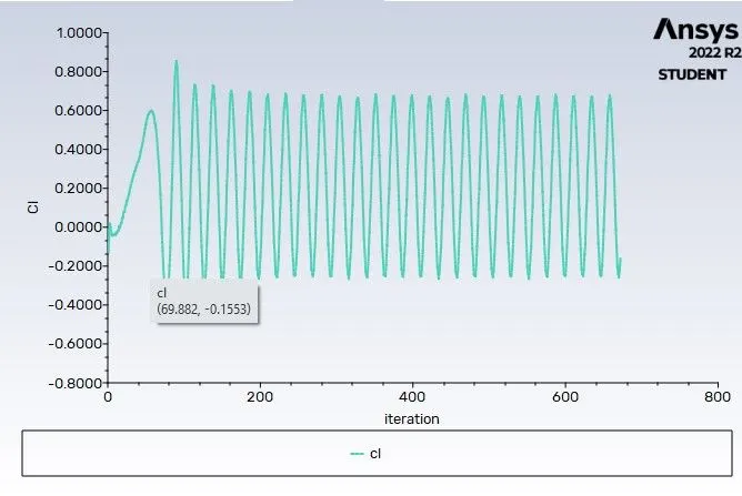
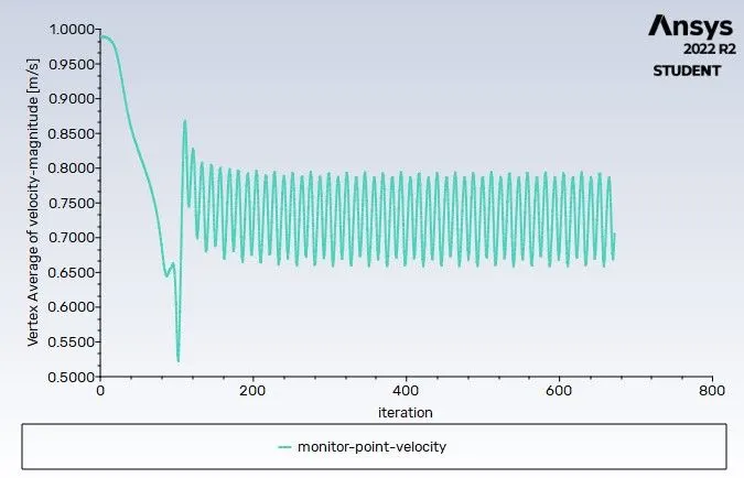
Case 3: Steady case with Re = 1000
a. Velocity Contour
b. Coefficient of Drag
c. Coefficient of Lift
d. Vertex average velocity at monitor point
e. Computed values of Coeff. of drag and Coeff. of lift
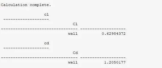
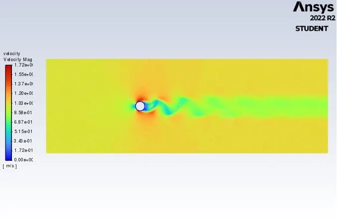
Case 4: Steady case with Re = 10000
a. Velocity Contour
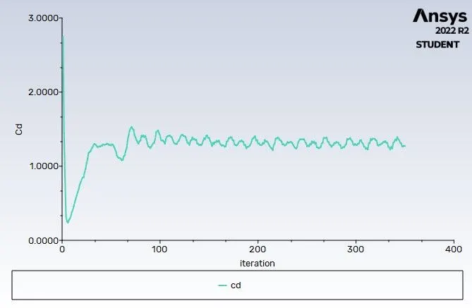
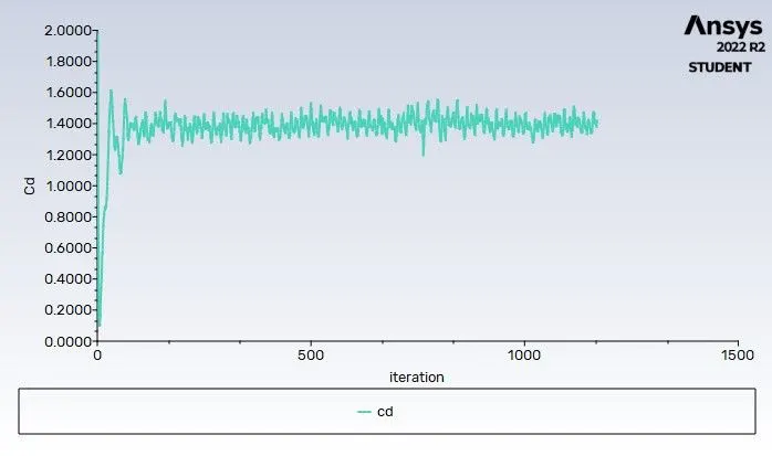
b. Coefficient of Drag
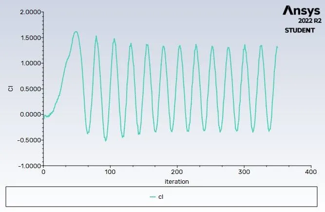
c. Coefficient of Lift
d. Vertex average velocity at monitor point
e. Computed values of Coeff. of drag and Coeff. of lift
Case 5: Steady case with Re = 100000
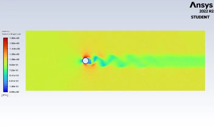
a. Velocity Contour
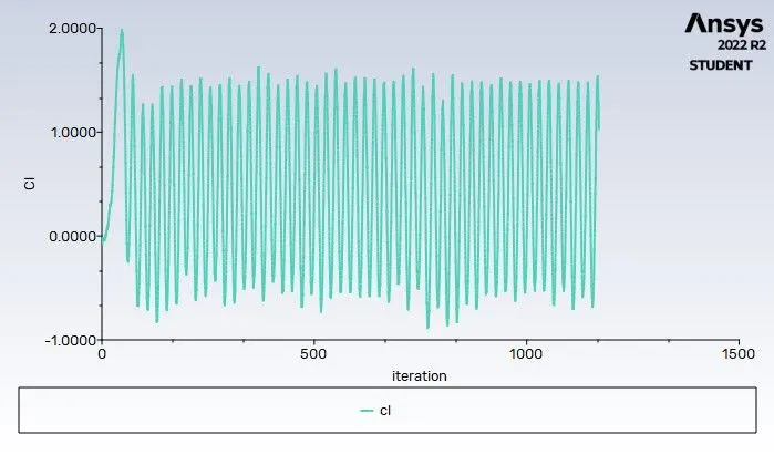
b. Coefficient of Drag
c. Coefficient of Lift
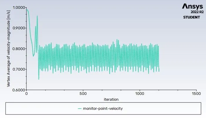
d. Vertex average velocity at monitor point
e. Computed values of Coeff. of drag and Coeff. of lift
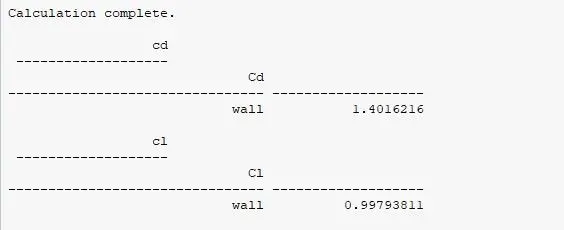
The table below shows the comparison of coefficient of drag and lift of each the cases in Part 2.
| Coefficient of Drag | Coefficient of Lift |
Coefficient of Drag[1] |
Coefficient of Lift[1] | |
|
Case 1 (Re = 10) |
5.427 | 0.0013 | ||
|
Case 2 (Re = 100) |
2.183 | 0.195 | 1.335 | 0.179 |
|
Case 3( Re = 1000) |
1.205 | 0.629 | ||
|
Case 4 (Re = 10000) |
1.27 | 1.297 | ||
|
Case 5 (Re = 100000) |
1.401 | 0.997 |
From the table it is clear Coeff of drag increases with increase Reynolds number and coeff of lift decreases with increase Reynolds number. The same was observed in the referred journal.
CONCLUSION:
A study has been carried out on a flow over a cylinder model by using Ansys FLUENT. Simulation and comparison of different cases mentioned in questions are also done.
Link to videos: https://drive.google.com/drive/folders/1ftsbSn3l483jly2vmc1iIYOkaDi6jGtr?usp=sharing
REFERENCE:
[1] https://www.sciencedirect.com/science/article/pii/S0307904X08000243