Week 2 - Flow over a Cylinder.
AIM:- To simulate flow past a cylinder with varying Reynolds number
Objective:-
- To understand the Karman vortex street phenomenon.
- Simulate the steady and unsteady (transient) cases for a range of Reynolds numbers.
- To calculate and validate the drag and lift coefficient at different Reynolds numbers.
- To calculate the Strouhal number for the unsteady case.
Introduction:-
The flow past a 2-D cylinder is one of the most studied of aerodynamics. It is relevant to many engineering applications. The flow pattern and the drag on a cylinder are functions of the Reynolds number, based on the cylinder diameter D and the undisturbed free-stream velocity U.
- Consider laminar fluid flows over a circular cylinder for steady and unsteady cases. Fluid flow analysis aims to determine the relationship between pressure and flow velocity which is subject to a geometric boundary condition, i.e., the interface surface at which a fluid contacts a solid object.
- At the leading edge of the cylinder, a stagnation point is formed where the oncoming flow is at rest. The pressure at this point is called stagnation pressure. To either side of the stagnation point, the flow accelerates around the forward surface of the cylinder producing a drop in pressure.
- A thin boundary layer is formed to the adjacent side of the cylinder surface, there is zero fluid velocity (i.e., no-slip) is achieved over the whole surface of a solid object.
-At a low Reynolds number Re< 400000 the boundary layer remains laminar(it depends upon the shape of the body and free stream velocities for external flow cases) from the stagnation point at the front of the cylinder to the point where it separates.
- Due to adverse pressure gradient the laminar boundary detaches from the body and flow separation takes place.
- Downstream of separation the flow quickly becomes turbulent and a broad wake is formed. The wake as a whole is unstable and rolls up into vortices that are shed unsymmetrically at regular intervals from the cylinder. This type of wake is called a Karman vortex street.
- Because of separation, the pressure remains low and approximately constant over the rearward face of the cylinder. This causes a net imbalance of pressure forces on the cylinder, usually referred to as pressure drag.
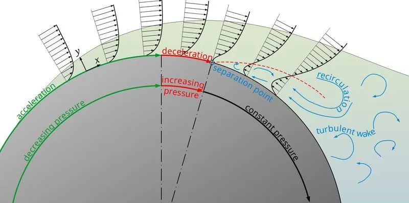
- At Reynolds number greater than the critical value (generally Re> 400000) the boundary layer on the forward face of the cylinder undergoes a transition and becomes turbulent.
Von Karman vortex street- A von Karman vortex street is a repetitive pattern of swirling vortices, caused by a process known as vortex shedding. (Vortex shedding is an oscillating flow that takes place when fluid flows over a bluff body at certain velocities. In this flow vortices are created at the back of the body (wake region) that detach periodically from either side of the body.)
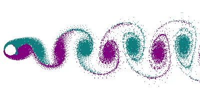
Though vortex shedding is an unsteady phenomenon occurring in laminar flows, the frequency of steady vortex shedding is observed at Re = 100. In order to calculate the frequency at which vortex are been shed, a dimensionless number called "Strouhal number" is used.
Strouhal number- The Strouhal number is a dimensionless value useful for analyzing oscillating unsteady fluid flow dynamics problems.
It represents a measure of the ratio of inertial forces due to unsteadiness of the flow or local acceleration to inertial forces due to changes in velocity from one point to another in the flow field.
The Strouhal number is calculated only for transient simulations. Because of its time-accurate approximation & is given by the following expression.
`St = (omega l)/v`
- where,
`omega` is the oscillation frequency.
l is the Characteristics length
v is the flow velocity
Co-efficient of drag- It's a dimensionless quantity that is used to quantify the drag or resistance of an object in a fluid environment, such as air or water. It is used in the drag equation in which a lower drag coefficient indicates the object will have less aerodynamic or hydrodynamic drag. The drag coefficient is always associated with a particular surface area.
`C_d=(2F)/(ρAV^2)`
where,
F - Drag force.
`C_d` - Drag coefficient.
`rho` - Density of fluid.
A - Area of the object facing the fluid.
V - Velocity of the fluid.
Co-efficient of lift - The lift coefficient (CL) is a dimensionless coefficient that relates the lift generated by a lifting body to the fluid density around the body, the fluid velocity, and an associated reference area. A lifting body is a foil or a complete foil-bearing body such as a fixed-wing aircraft. CL is a function of the angle of the body to the flow, its Reynolds number, and its Mach number. Lift is the component of this force that is perpendicular to the oncoming flow direction. It contrasts with the drag force, which is the component of the force parallel to the flow direction. Lift conventionally acts in an upward direction in order to counter the force of gravity, but it can act in any direction at right angles to the flow.
`Cl=(L)/(0.5*A*r*V^2)`
The quantity one-half the density times the velocity squared is called the dynamic pressure q. So
`Cl=(L)/(q*A)`
The lift coefficient then expresses the ratio of the lift force to the force produced by the dynamic pressure times the area.
Cases-
Case 1- Simulate the flow with the steady and unsteady case for Re= 100.
Case 2- Calculate the coefficient of drag and lift over a cylinder by setting the Reynolds number
`Re = (uL)/v`
where,
u is the flow speed (m/s)
L is a characteristic linear dimension (m)
v is the fluid flow velocity
| Reynold's number | Velocity of the fluid (m/sec) |
| Re = 10 | 0.25 |
| Re = 100 | 2.5 |
| Re = 1000 | 25 |
| Re = 10000 | 250 |
| Re = 100000 | 2500 |
Assume-
An artificial fluid is created to visualize the viscous flow over a cylinder. The flow will remain incompressible and viscosity will remain constant for all the cases. To attain desired Reynolds number, velocity will be modified for the respective cases.
| Fluid | User-Defined |
| Density | 1 kg/`m^3` |
| Viscosity | 0.05 kg/m-s |
Procedure-
Geometry- Initially cylinder geometry is created in Spaceclaim and the appropriate flow volume region is created defined as a surrounding to a cylinder.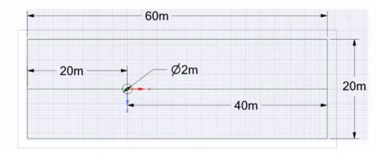
Creating Surface Domain for flow around the cylinder
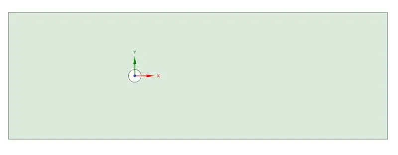
Mesh-
Boundary condition- First, we will name the edges as inlet, outlet, symmetry, and cylinder wall.
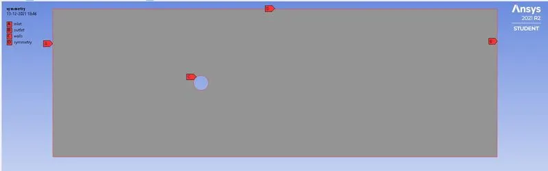
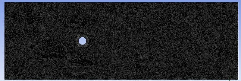
Mesh- We create our baseline mesh, then refine the mesh as the 'All triangles method', the element size is kept at 0.1m.
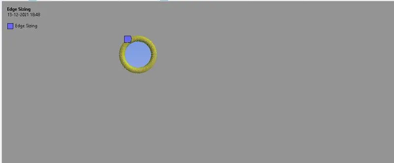
Sizing - In automatic mesh generation, cylinder boundary is affected resulting in the non-circular wall at the boundaries. Because of this the flow field calculation and analysis gets affected drastically
To get a perfect cylinder shape(circle as it is 2D) sufficient for our case we need to increase the no. of divisions to 80 of the circle
Inflation- Inflation is an important aspect in meshing the geometry to capture the flow field at the wall conditions.
Here we use first layer thickness 0.01 mm and numbers of layers = 8. The layer size increases from layer to layer depending upon the growth ratio we give. Here we put the growth ratio as 1.2.
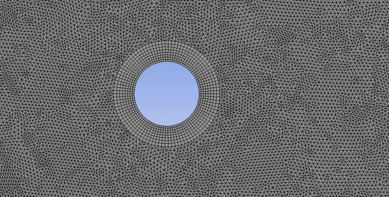
Resulting mesh- The element size is set to be 0.1m which results in 250786 elements.
Setup-
Solver type- Pressure based
Time- steady-state / Transient State
velocity formulation -absolute
viscous model -laminar
Pressure-velocity coupling method: SIMPLE (Semi-Implicit Method for Pressure Linked Equations)
Material - User-Defined having Density 1 kg/`m^3` and viscosity 0.05 kg/m-s
Boundary Condition-
Inlet- velocity is 1 m/sec
Outlet - pressure outlet is gauge pressure = 0 pa
Cylinder wall - wall having no slip property
Other set-up characteristics
- Monitor point- We want to see the vortex average at a point, for that we need a monitor point, we have to create a point. The monitor point is a point in space at which flow quantities can be approximated.
In this particular case, 4*Diameter = 4*2 = 8m at which the monitor point is specified.
- Now we also want to monitor the lift and drag coefficient plot while the solution is being run. Create lift and drag coefficients plots.
- Also we want to monitor the lift and drag coefficient plot while the solution is being run. Create lift and drag coefficients plots.
- Animation setup is made as the solution is changing as the function of time we can see the physics behind it.
- Pressure and velocity contours is being generated.
Solution-
Case 1- Simulate the flow with the steady and unsteady case for Re= 100.
Residual graphs- to check the solution how much numerically accurate
Steady State 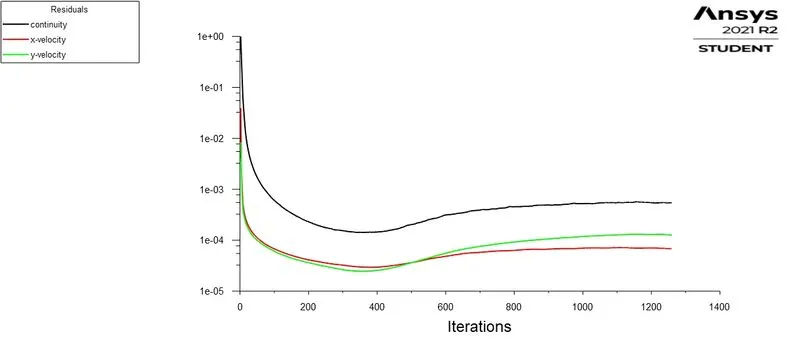 |
Transient State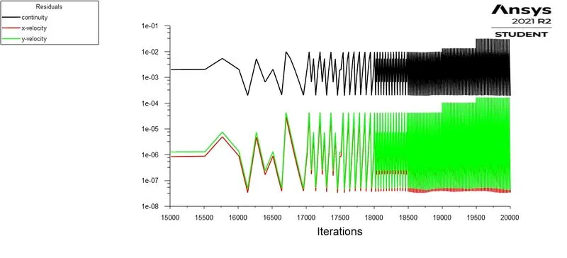 |
Velocity fluctuations at a specified monitor point
Steady State 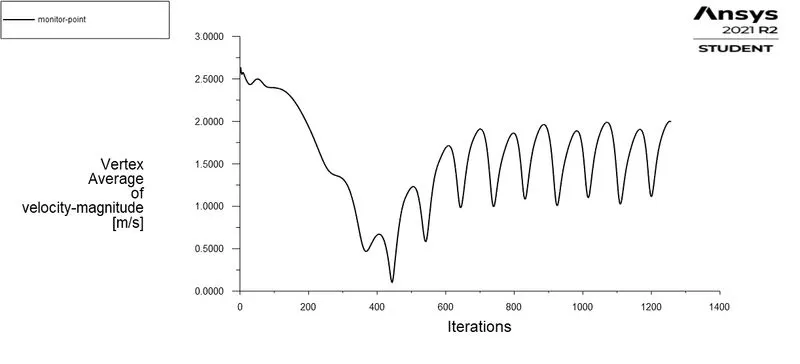 |
Transient State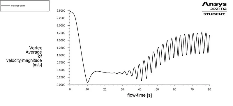 |
Coefficient of drag (cd)
Steady State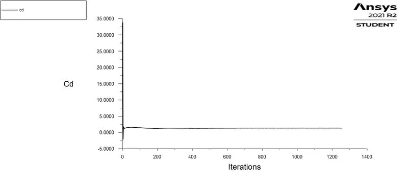 |
Transient State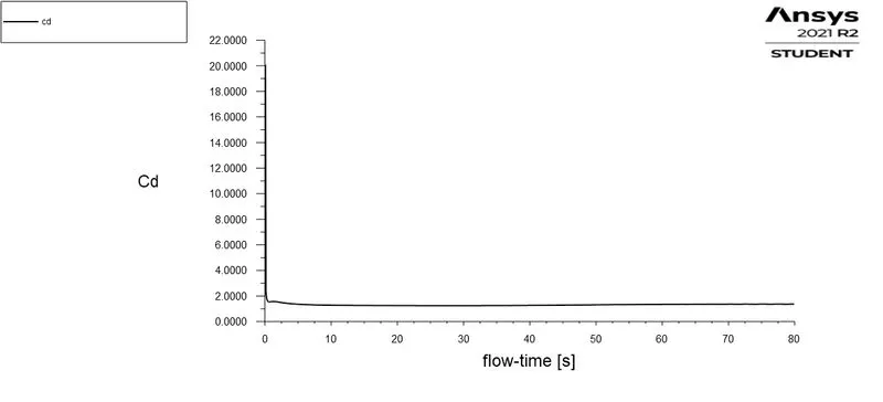 |
Coefficient of lift (cl)
Steady State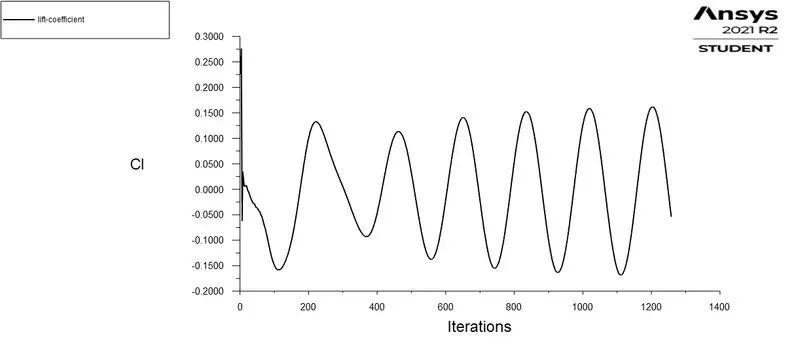 |
Transient State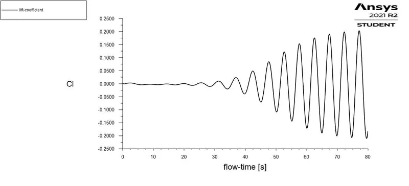 |
Report Definitions
Steady State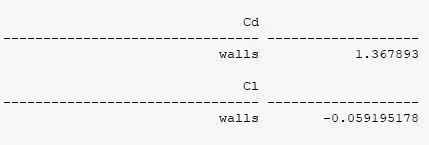 |
Transient State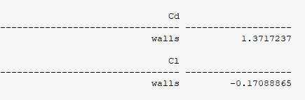 |
Comparison of drag co-efficient for Reynolds number 100
| Condition | Analytical value | Numerical value | Error(%) |
| Steady-state | 1.347501 | 1.3678930 | 1.46 |
| Unsteady state | 1.3717237 | 1.52 |
From the above table, it is clear that the numerical value closely matches the analytical value and the error is within 5% for both cases.
Contour Plots-
Pressure contour
Steady State 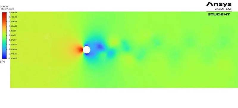 |
Transient State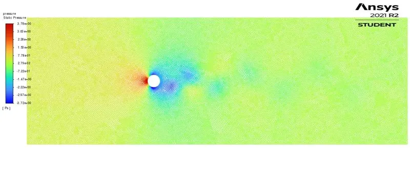 |
Velocity contour
Steady State 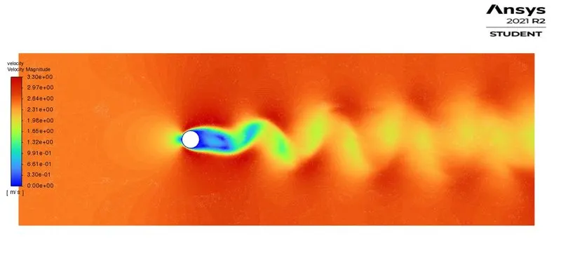 |
Transient State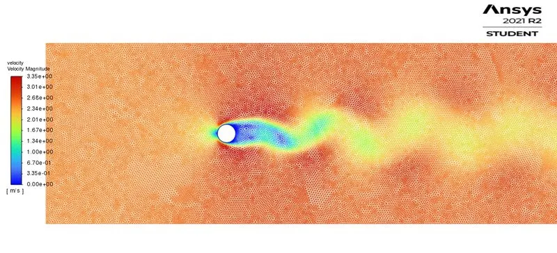 |
Velocity vector contour
Steady State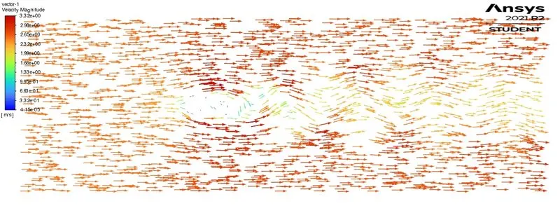 |
Transient State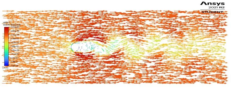 |
Velocity pathlines contour
Steady State 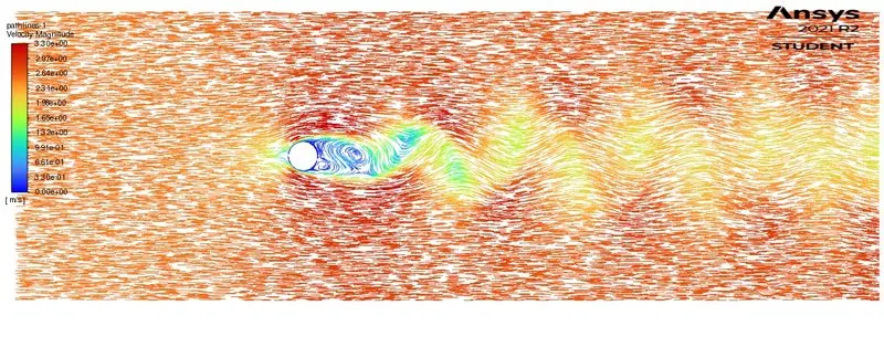 |
Transient State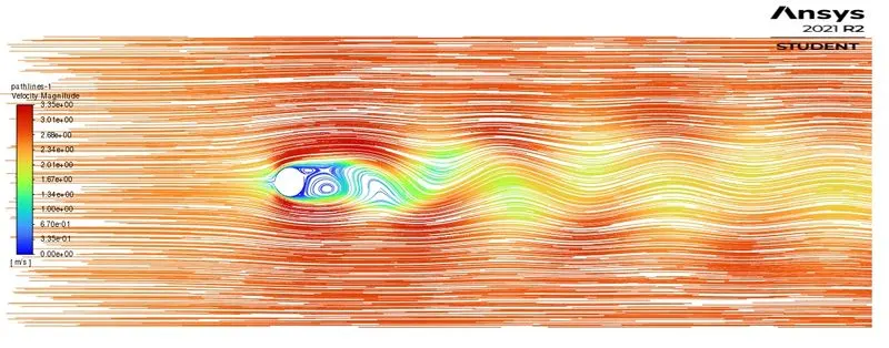 |
Observation from these Plots:-
- If we compare the velocity contour plots for the steady and unsteady state there is not much difference but the velocity contour looks more realistic in the transient state so, we prefer transient state simulation.
- The coefficient of lift becomes almost constant after the 250 iterations in steady-state and In the unsteady state, it fluctuates at every time step.
- Coefficient of discharge is constant for both steady and unsteady simulation but the average cd value for steady-state is 1.318 and for the transient state is 1.46.
- In a steady-state, the residual plot isn't oscillating when you increase the number of iterations but in the unsteady state iterations increasing oscillation starts fluctuating.
- In a steady-state, the velocity with respect to iteration is slowly as compared to the transient state.
Strouhal number
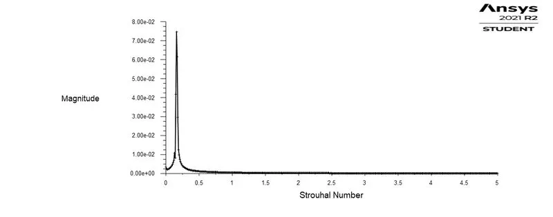
| Numerical Strouhal number | Analytical strouhal number |
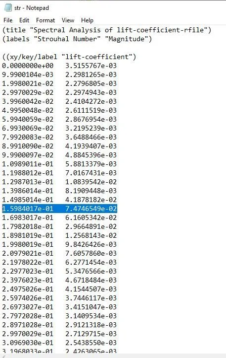 |
Strouhal = `(omega L)/v` `omega` = No. of oscillations/Time difference `omega = 2/10` Strouhal = `((2/10)*2)/2.5` = 0.016 |
From the above table, it is clear that the analytically calculated Strouhal number equals the numerical Strouhal number. Thus it is verified.
Case 2- Calculate the coefficient of drag and lift over a cylinder by setting the Reynolds number
| Reynold's number | Velocity of the fluid (m/sec) |
| Re = 10 | 0.25 |
| Re = 100 | 2.5 |
| Re = 1000 | 25 |
| Re = 10000 | 250 |
| Re = 100000 | 2500 |
Setup-
Solver type- Pressure based
Time- steady-state
Velocity formulation -Absolute
Viscous model -Laminar
Pressure-velocity coupling method: SIMPLE (Semi-Implicit Method for Pressure Linked Equations)
Material - User-Defined having Density 1 kg/`m^3` and viscosity 0.05 kg/m-s
Boundary Condition-
Inlet- velocity is 1 m/sec
Outlet - pressure outlet is gauge pressure = 0 pa
Cylinder wall - wall having no slip property
Solution-
Residual graphs- to check the solution how much numerically accurate
|
Re = 10 and velocity 0.25m/s |
| Re = 100 and velocity 2.5m/s |
Re = 1000 and velocity 25m/s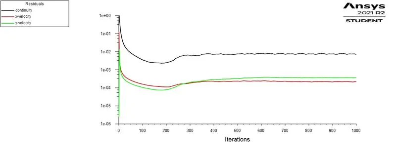 |
Re = 10000 and velocity 250m/s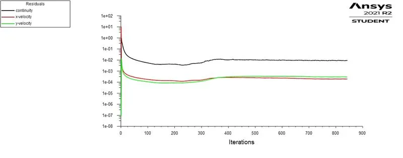 |
Re = 100000 and velocity 2500m/s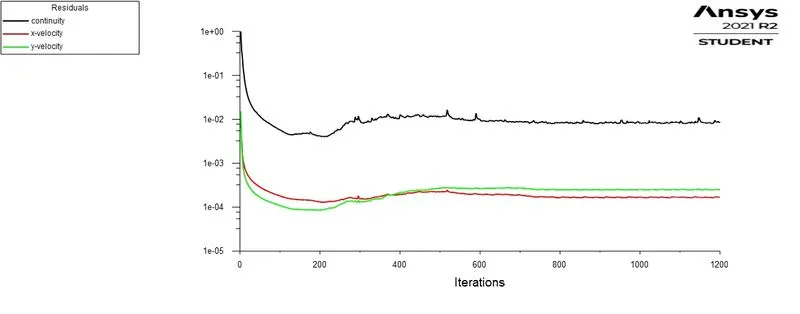 |
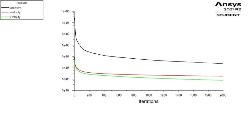
Velocity fluctuations at a specified monitor point
Re = 10 and velocity 0.25m/s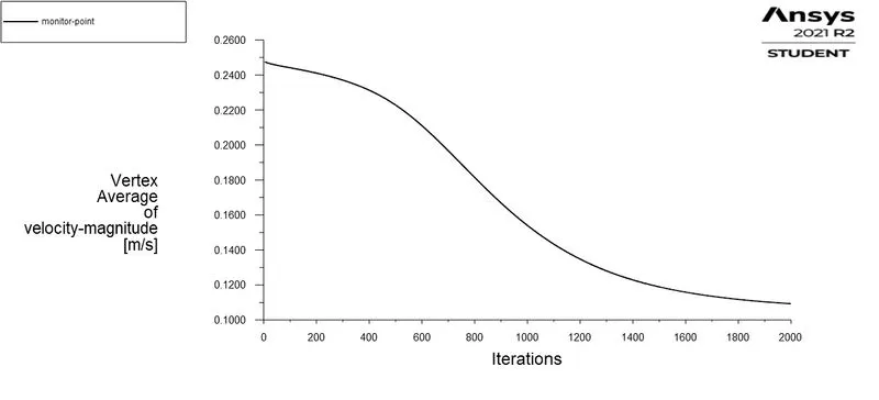 |
| Re = 100 and velocity 2.5m/s |
Re = 1000 and velocity 25m/s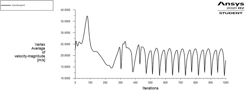 |
Re = 10000 and velocity 250m/s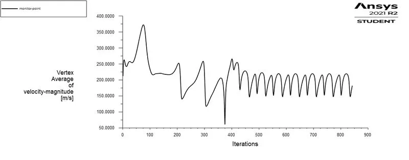 |
Re = 100000 and velocity 2500m/s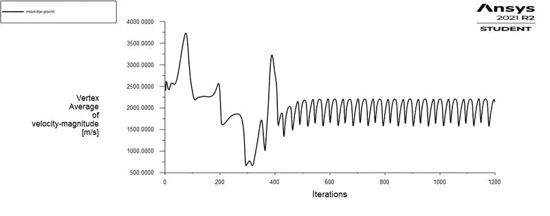 |
Coefficient of drag (cd)
Re = 10 and velocity 0.25m/s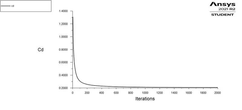 |
| Re = 100 and velocity 2.5m/s |
Re = 1000 and velocity 25m/s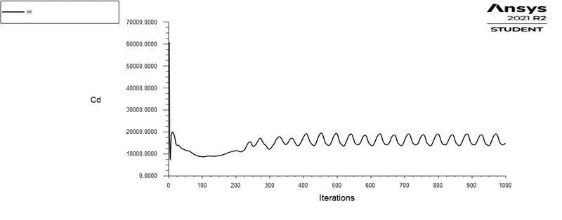 |
Re = 10000 and velocity 250m/s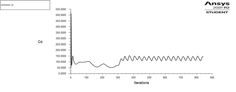 |
Re = 100000 and velocity 2500m/s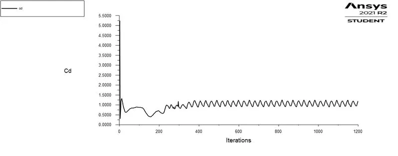 |
Coefficient of lift (cl)
Re = 10 and velocity 0.25m/s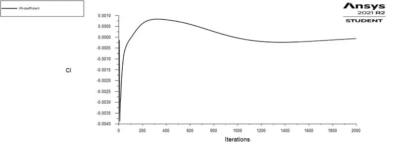 |
| Re = 100 and velocity 2.5m/s |
Re = 1000 and velocity 25m/s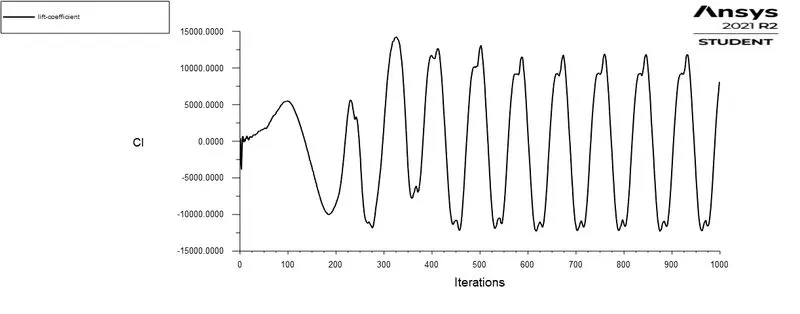 |
Re = 10000 and velocity 250m/s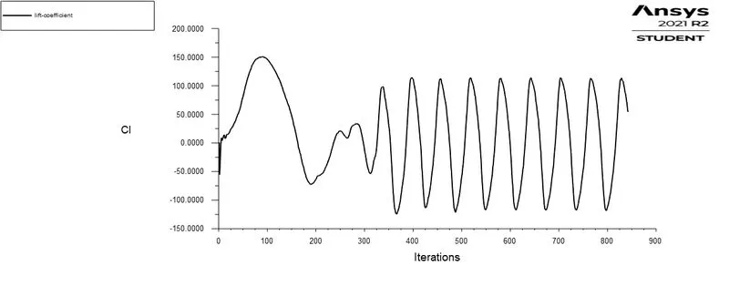 |
Re = 100000 and velocity 2500m/s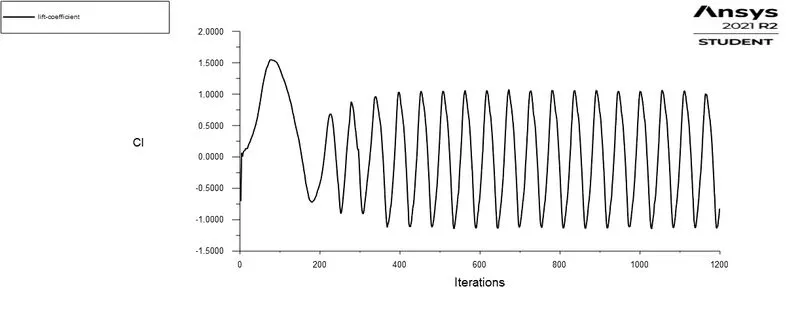 |
- From the table, we can observe that the drag coefficient decreases with the increase in the Reynolds number. An increase in Reynolds number leads to vortex shedding at the upper and lower side of a cylinder surface.
Contour Plots-
Pressure contour
Re = 10 and velocity 0.25m/s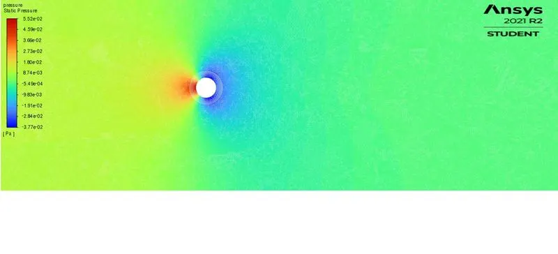 |
| Re = 100 and velocity 2.5m/s |
Re = 1000 and velocity 25m/s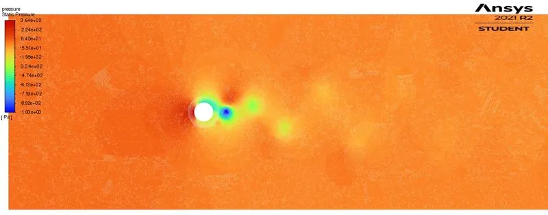 |
Re = 10000 and velocity 250m/s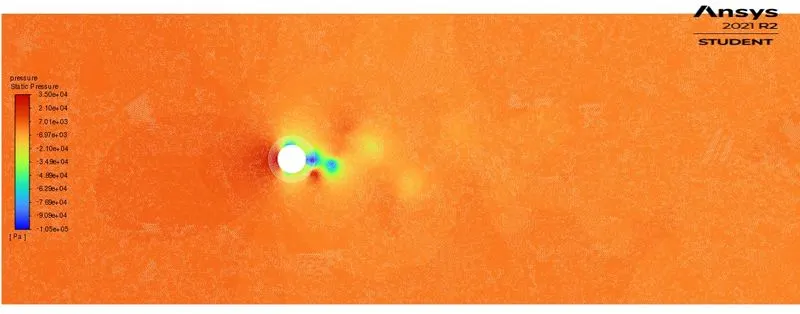 |
Re = 100000 and velocity 2500m/s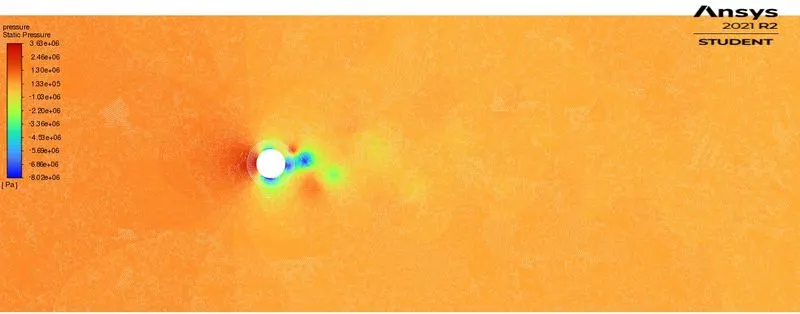 |
Velocity contour
Re = 10 and velocity 0.25m/s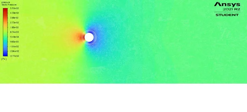 |
| Re = 100 and velocity 2.5m/s |
Re = 1000 and velocity 25m/s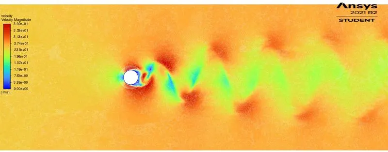 |
Re = 10000 and velocity 250m/s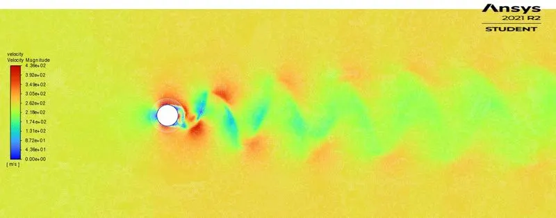 |
Re = 100000 and velocity 2500m/s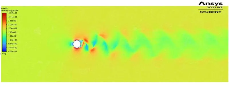 |
Conclusion
- Flow over a cylinder is successfully simulated and the effect of phenomena Karman vortex street is successfully analyzed for various conditions and for the various Reynolds number and the result are discussed above.
- Vortex shedding takes place when the Reynolds number is greater than or equal to 40(Re>40).
- In Reynolds number less than 40 there is no formation of vortices.
- In comparing steady-state and unsteady-state conditions. Unsteady state condition produces accurate results. Since the term vortex, Karman street is time-dependent.
Reference-
https://eng-web1.eng.famu.fsu.edu/~shih/succeed/cylinder/cylinder.htm
https://www.sciencedirect.com/science/article/pii/S0307904X08000243