Week 2 - Flow over a Cylinder.
AIM:- To Simulate the flow over a cylinder and explain the phenomenon of Karman vortex street.
OBJECTIVE:-
- Simulate the flow with the steady and unsteady case and calculate the Strouhal Number for Re= 100 and show that the flow has converged for both approches.
- Calculate the coefficient of drag and lift over a cylinder by setting the Reynolds number to 10,100,1000,10000 & 100000 and Discuss the effect of Reynolds number on the coefficient of drag.
- Plots of the coefficient of drag and lift and also show vortex shedding plot behind the cylinder.
Theory:- Consider laminar fluid flows over a circular cylinder for steady and unsteady cases. Fluid flow analysis aims to determine the relationship between pressure and flow velocity which is subject to a geometric boundary condition, i.e., the interface surface at which a fluid contacts a solid object. As very small uneven roughness is unavoidably distributed over the whole surface of a solid object, fluid particles are completely captured on the solid surface due to the viscosity of the fluid. This property of fluids leads to a very important assumption such that a condition of zero fluid velocity (i.e., no slip) is achieved over the whole surface of a solid object.
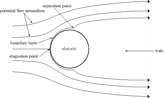
Whenever there is relative movement between a fluid and a solid surface, whether externally round a body, or internally in an enclosed passage, a boundary layer exists with viscous forces present in the layer of fluid close to the surface. Boundary layers can be either laminar or turbulent.
- Stagnation point is formed at the leading edge.
- Boundary layer remains laminar from stagnation point to the point where it seprates.
- Wake as a whole is unstable and rolls up into vortices that are shed anti-symmetrically at regular intervals from the cylinder.
Flow separation or boundary layer separation is the detachment of a boundary layer from a surface into a wake. Separation occurs in flow that is slowing down, with pressure increasing, after passing the thickest part of a streamline body or passing through a widening passage, for example.
Flowing against an increasing pressure is known as flowing in an adverse pressure gradient. The boundary layer separates when it has travelled far enough in an adverse pressure gradient that the speed of the boundary layer relative to the surface has stopped and reversed direction. The flow becomes detached from the surface, and instead takes the forms of eddies and vortices. The fluid exerts a constant pressure on the surface once it has separated instead of a continually increasing pressure if still attached. In aerodynamics, flow separation results in reduced lift and increased pressure drag, caused by the pressure differential between the front and rear surfaces of the object.
The relative importance of the ratio of the inertial forces to the viscous forces for the flow conditions is quantified by taking L as the characteristic scale of flow and U as characteristic velocity of flow
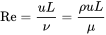
where:
- ρ is the density of the fluid (SI units: kg/m3)
- u is the flow speed (m/s)
- L is a characteristic linear dimension (m) (see the below sections of this article for examples)
- μ is the dynamic viscosity of the fluid (Pa·s or N·s/m2 or kg/(m·s))
- ν is the kinematic viscosity of the fluid (m2/s).
If the Navier-Stokes Equation is converted to a dimensionless form, it is well known that this dimensionless equation depends on only the Reynolds number. Thus, if Reynolds numbers are identical, an overall field containing every individual flow with a geometrically similar boundary shape to each other can be regarded as being similar overall. In addition to increasing velocity, a greater density, a smaller viscosity, or a larger solid body size tend to increase the Reynolds number, thereby equally affecting the overall flow field. Accordingly, it can be said that the Reynolds number represents a dimensionless flow velocity. As the Reynolds number increases, the length of the vortex increases. When the Reynolds number exceeds 60, the rear flow becomes unstable and the vortex begins to oscillate in an up-down direction. The fully formed vortex is carried away on the surrounding
main flow, and a vortex subsequently occurs on the other side. This vortex then expands before finally dissipating and departing leaving the circular cylinder. In addition to this flow process, every pair of upper and lower vortices behind the cylinder is stored in an alternative regular array to form twin rows of vortices. These rows are called the von Karman vortex street.
In fluid dynamics, a Kármán vortex street (or a von Kármán vortex street) is a repeating pattern of swirling vortices, caused by a process known as vortex shedding, which is responsible for the unsteady separation of flow of a fluid around blunt bodies. A vortex street will form only at a certain range of flow velocities, specified by a range of Reynolds numbers (Re), typically above a limiting Re value of about 90. The (global) Reynolds number for a flow is a measure of the ratio of inertial to viscous forces in the flow of a fluid around a body or in a channel, and may be defined as a nondimensional parameter of the global speed of the whole fluid flow:The perfect visualization of the vortex streets while flow fluid over a cylinder.
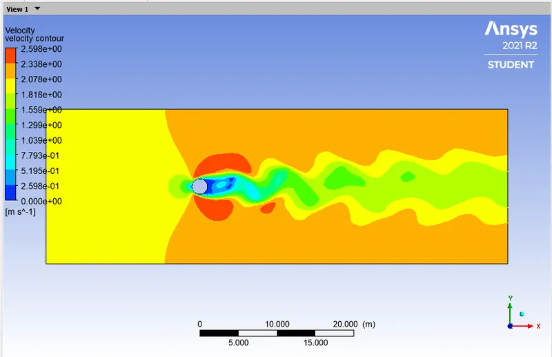
vortex shedding:- In fluid dynamics, vortex shedding is an oscillating flow that takes place when a fluid such as air or water flows past a bluff (as opposed to streamlined) body at certain velocities, depending on the size and shape of the body. In this flow, vortices are created at the back of the body and detach periodically from either side of the body forming a Von Kármán vortex street.
Strouhal number:-
In flows characterized by a periodic motion, the Strouhal number is associated with the oscillations of the flow due to the inertial forces relative to the changes in velocity due to the convective acceleration of the flow field. Thus, an alternative definition of the Strouhal number better suited to periodic flows is given by the following expression.

- where,
f is the frequency of the oscillations with dimensions T-1. Best examples of such oscillations are found in vortex street wakes behind bluff bodies. When the velocity and pressure fields are calculated, the drag and lift coefficients, as well as the Strouhal number can also be determined. This can be performed using directly the force field or through the following relations:

where:
 is the drag force, which is by definition the force component in the direction of the flow velocity
 is the mass density of the fluid
 is the flow speed of the object relative to the fluid,
 is the reference area.
- The drag force equation
-

- is essentially a statement that the drag force on any object is proportional to the density of the fluid and proportional to the square of the relative flow speed between the object and the fluid.
 is not a constant but varies as a function of flow speed, flow direction, object position, object size, fluid density and fluid viscosity. Speed, kinematic viscosity and a characteristic length scale of the object are incorporated into a dimensionless quantity called the Reynolds number
  .
.  is thus a function of . In a compressible flow, the speed of sound is relevant, and is also a function of Mach number
  .
.
Coefficient of lift:- The lift coefficient (CL) is a dimensionless coefficient that relates the lift generated by a lifting body to the fluid density around the body, the fluid velocity and an associated reference area. A lifting body is a foil or a complete foil-bearing body such as a fixed-wing aircraft. CL is a function of the angle of the body to the flow, its Reynolds number and its Mach number. Lift is the component of this force that is perpendicular to the oncoming flow direction. It contrasts with the drag force, which is the component of the force parallel to the flow direction. Lift conventionally acts in an upward direction in order to counter the force of gravity, but it can act in any direction at right angles to the flow.

where
 is the lift force
- is the air density
 is the velocity or true airspeed
 is the planform (projected) wing area (in aerodyamics).
 is the lift coefficient at the desired angle of attack, Mach number, and Reynolds number.
Solving approch:-
We are going to capture the flow patterns or behaviour with every regime It is important to have a Renolds number is greater than the 40-48, velocity is approx 2.5 m/s and mesh size is less than the 0.25 or you can say that less mesh size too see the vortex shedding phenonena detach periodically from either side of the body forming a Von Kármán vortex street.
In this problem we have to solve for both cases steady and unsteady flow. In the steady state solver simulation took with the varying in renolds number and the whole property is remains constant. The problem we will start with 2D geometry of the flow field and less mesh size to capture the every little details of flow domain. The inflation layer will be also added near the cylinder to capture boundary layer detachment from the sureface of the Cylinder and It is also called body-fitted mesh.
In the Steady state solver we are going to use the SIMPLE Interpolation scheme to calculate the results in neighbouring Volume and for the Unsteady state solver we are going to use the SIMPLE Interpolation scheme and other one is PISO with NITA. This solver is more towards to solving time marching problems with less number of iterations. To check the convergence of solution we will create a monitor at a distance of 8 m behind the cylinder which will be used to plot the strouhal number and after that we will calculate the coefficient of drag and lift on the cylinder walls.
Case 1 :-Simulate the flow with the steady and unsteady case for velocity is 1 m/s and calculate the Strouhal Number for Re= 100
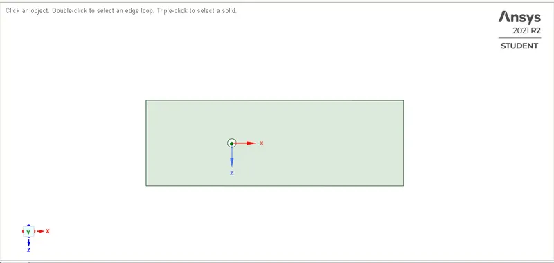
Step 1:- First we have create a 2D geometry form this sketch given below
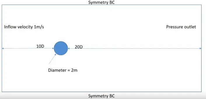
As you see in the above sketch there is a circular 2D cylinder which is immersed in the fluid domain and the inlet flow velocity is 1 m/s and the pressure outlet is 1 atm. We are going to use the inlet velocity is 2m/s to see the vortex shedding effect effciently. The given viscosity of this project is 1 pa but we are going to varry the velocity further for the different renolds number and velocity remains constant as 2 m/s.
Here, is the created 2D geometry. After creating a geometry use pull command to convert the fluid domain into the surface.
Step 2 :-Create Mesh
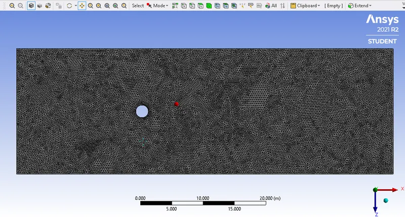
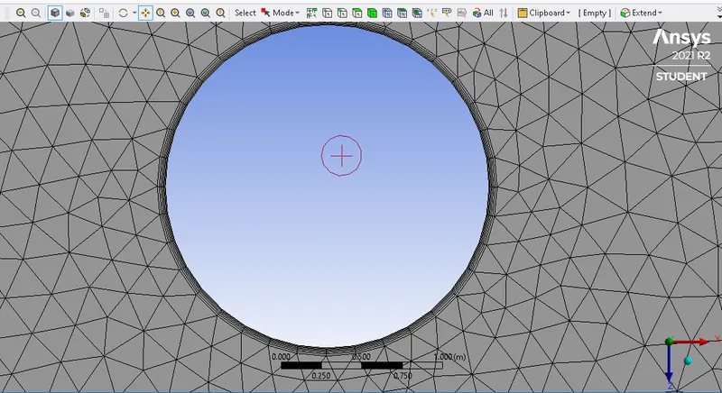
After creating a Geometry we are going to create Mesh and Meshing involves the creation of small dscreate domain for calculation of governing equations. In this we are using the Mesh element size is 0.25m for overall domain because we want to capture the every flow seperation point over a cylinder. To capture the the flow near the cylinder walls for that we are going to use inflation layer beacuse it is such body fitted mesh and the inflation will create a hexahedral mesh near the walls of the cylinder whereas, in the overall domain we are using the triangular mesh to get the accurate results at every point of fluid domain.
Mesh of element size 0.25m 6 Inflation layer of growth rate 1.2
Mesh quality
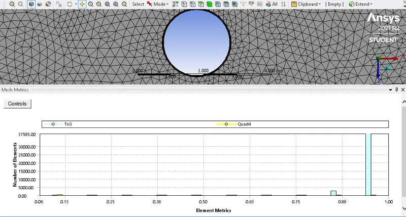
Before inserted the inflation layers we have to make the perfect cylinderical boundary by using the sizing method type we are using is no. of divisons to make it perfect circular boundary near the cylinderical surface. The inflation layer thickness in which the height we are using is about 5mm. No of inflation layers we are using is 6. In this we have quadratic and triangular mesh elements to get the solution convergence effciently and acurately.
Make sure FLUENT read the boundary conditions from workbech named selection should be provided accordng to flow parameters that is given in the challenge. The inlet, outlet and walls names is provided and also the boundarys are provided the name as symmetry.
Step 2 :-Start the Setup fluent
First you have to check the turbulence model that is we are using it in this case is Laminar flow because the Reynolds number for this case is less than 2000 and after that we have to check the material properties. Go to create materials then go to fluent base select the air as a fluent and then copy this as a new name user-material.
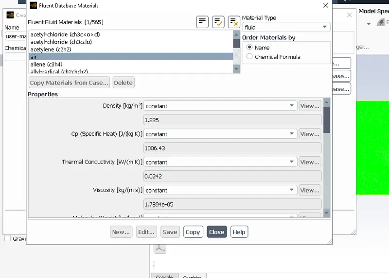
After that delete the all fluids expect the user-material that we are going to use it and put the valid values for density and viscosity.
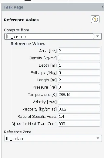
Now, we are going to give the Boundary conditions as inlet velocity is 1 m/s and the outlet pressure is 1 atm and After that we are going to give the Refrence values. Is is the most important seeting for the simulation is refrence value setting in the FLUENT. It will change the value with respect to the refrence frame from the previous value of updated value.
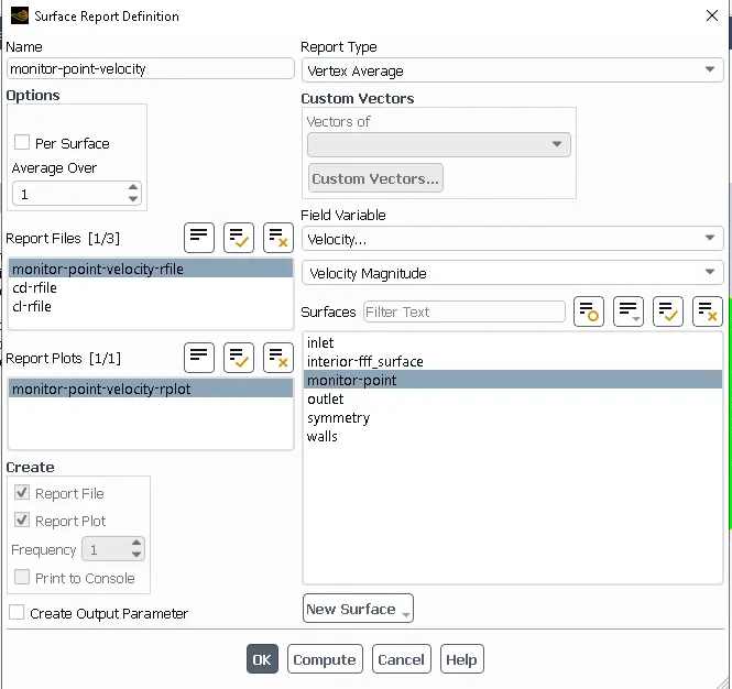
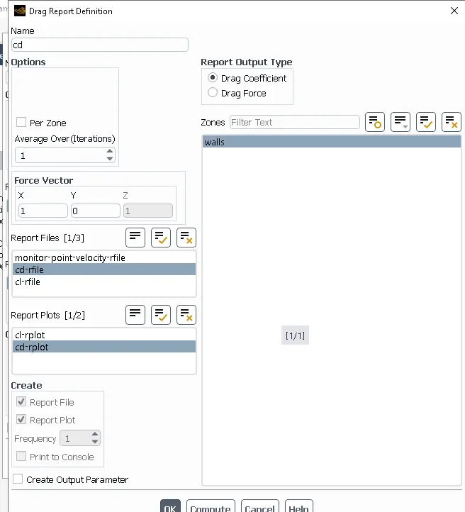
After that we have to create a monitor point where we want to capture the simulation or flow patterns or we can say that to capture the Vortex shedding behind the cylinder at a distance of 8m from the centre of the cylinder in x direction. The first report will be vertex average of velocity and its magnitude and then the coefficent of drag and lift. To get the contour plots of velocity and pressure we would write the report of area-weighted average report.
Vortex shedding report settings Coefficient of drag force report settings
Coeffcient of lift force settings Pressure and Velocity settings to get contour plots
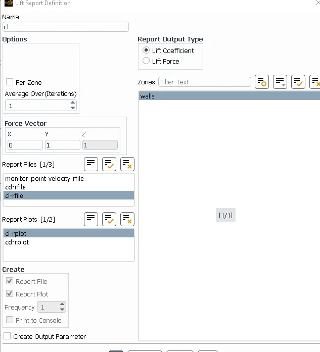
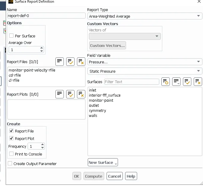
In this simulation we are using the SIMPLE interploation scheme
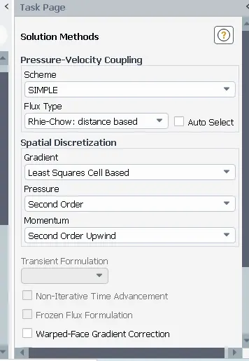
After setting up the whole project hit the calculate and we will get the results that is mentioned in below For the steady state we give the number of iterations and for the unsteady or transient state calculations we give the number of time steps as 500 and the step size is 0.01.
Results for steady state simulation for re = 100
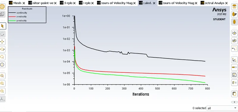
Residual plot
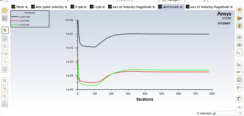
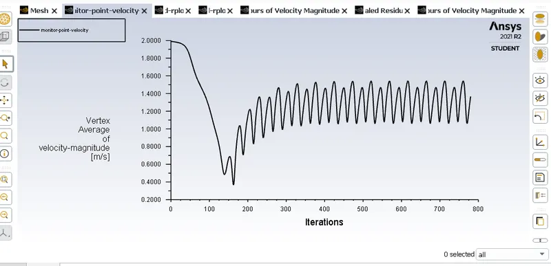
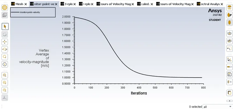
Vertex average of velocity magnitude
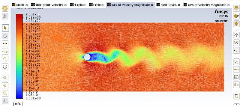
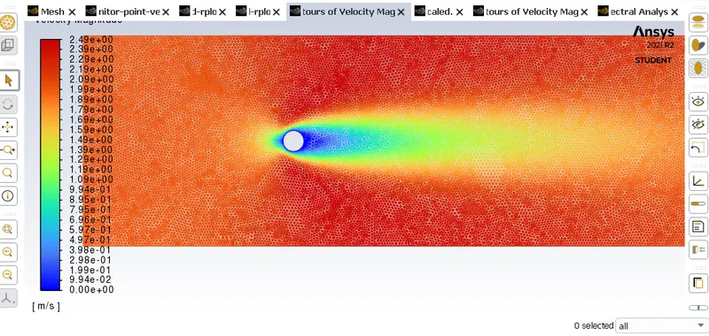
Velocity contour
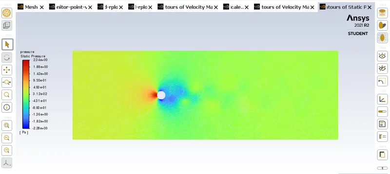
Pressure Contour Plot
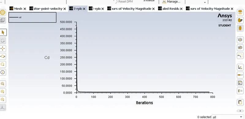
Coefficient of drag plot
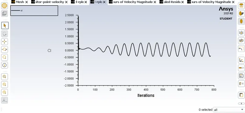
Coefficient of lift
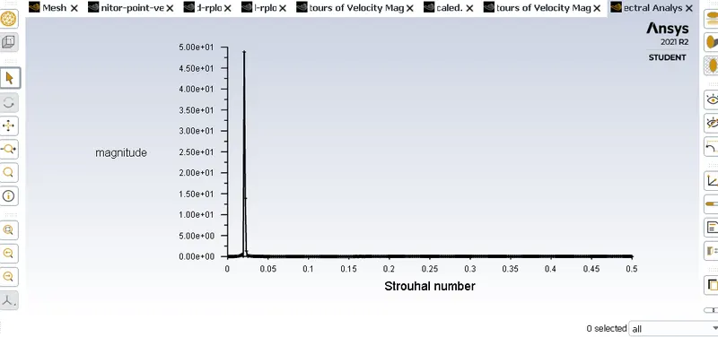
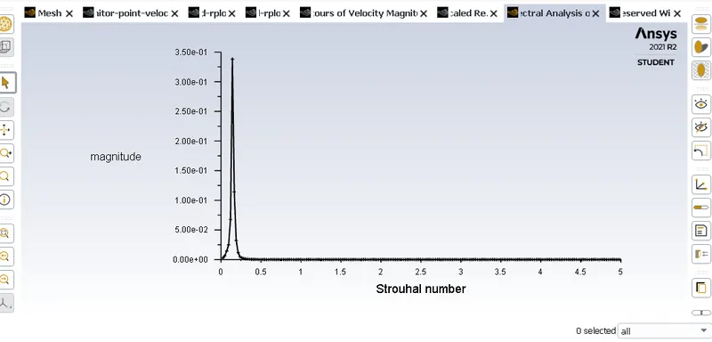
Strouhal number Plot
To know the strouhal number from the coefficient of lift data file for that we have to go in the FLUENT in which we have to choose the FFT option. After opening the FFT file the y axis is magnitude and the x axis is strouhal number data is given and then load the input file of coefficient of lift. The strouhal number is approx 5e1
Results for unsteady state simulation for re = 100
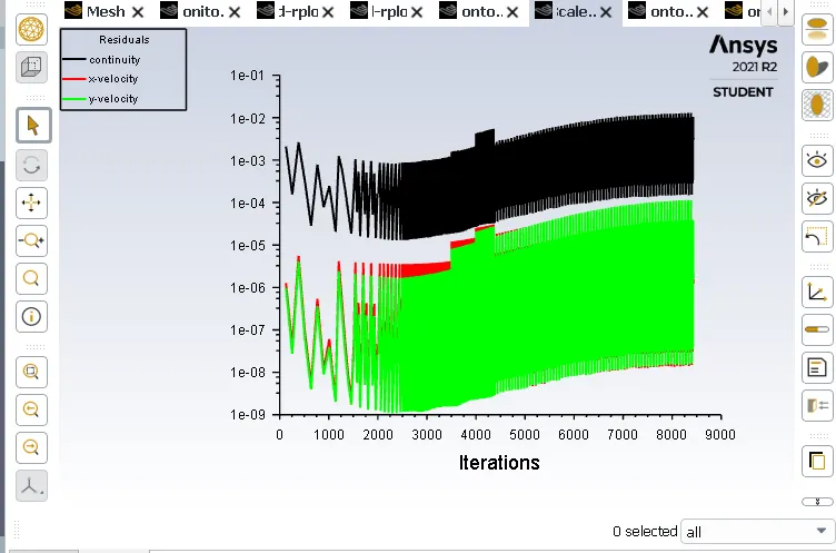
Residual plot
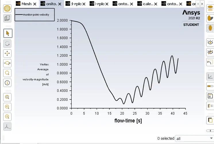
Vertex average of velocity magnitude
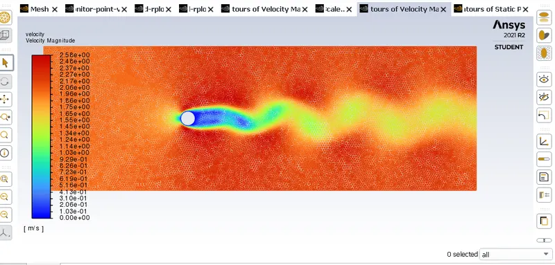
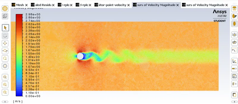
Velocity contour
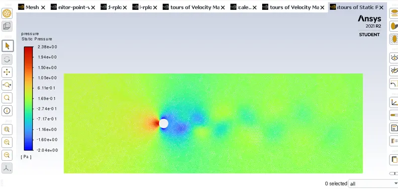
Pressure Contour Plot
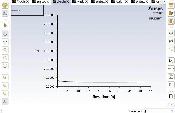
Coefficient of drag plot
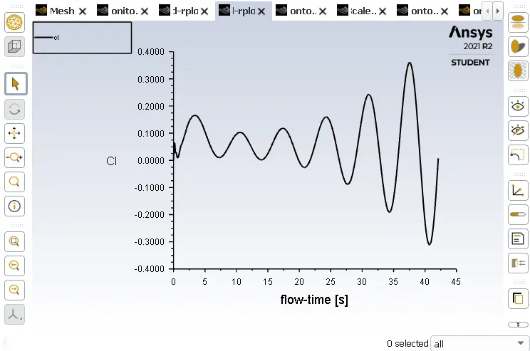
Coefficient of lift
Strouhal number Plot
strouhal number for unsteady state simulation is approx 0.348
Conclusion from these Plots:-
- If we compare the velocity contour plots for steady and un steady state there is no much difference but the velocity contour looks more realstic in transient state so, we prefer transient state simulation.
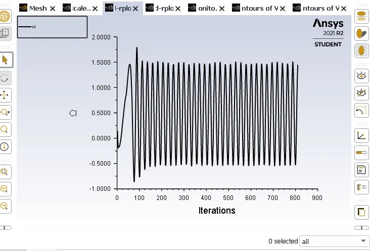
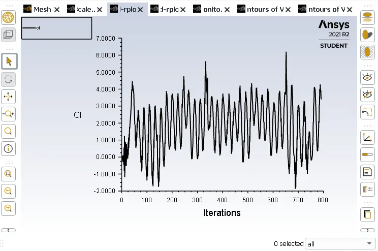
- The coeffcient of lift becomes almost constant after the 250 iterations in steady state and In unsteady state it fluctuating at every time step.
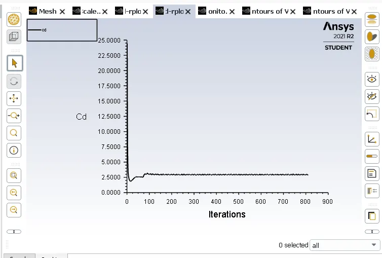
- Coefficient of discharge is constant for both steady and unsteady simulation but the average cd value for steady state is 1.318 and for transient state is 1.46.
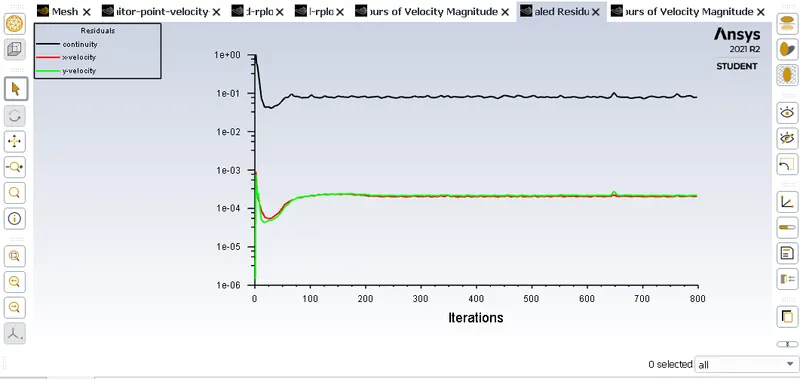
- In steady state the residual plot isn't oscillating when you increase the number of itertions but in the unsteady state iterations increasing oscillation starts fluctuating.
- In steady state the velocity with respect to iteration is slowly as compared to the transient state.
Case 2:- Simulate the flow of steady state case for velocity 1m/s and Calculate the coefficient of drag and lift over a cylinder by setting the Reynolds number to 10,100,1000,10000 & 100000 and also Discuss the effect of Reynolds number on the coefficient of drag.
Results for steady state simulation for re = 10
Residual plot
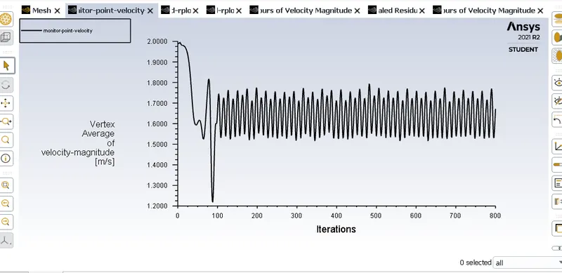
Vertex average of velocity magnitude
Velocity contour
Coefficient of drag plot
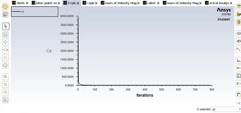
Coefficient of lift
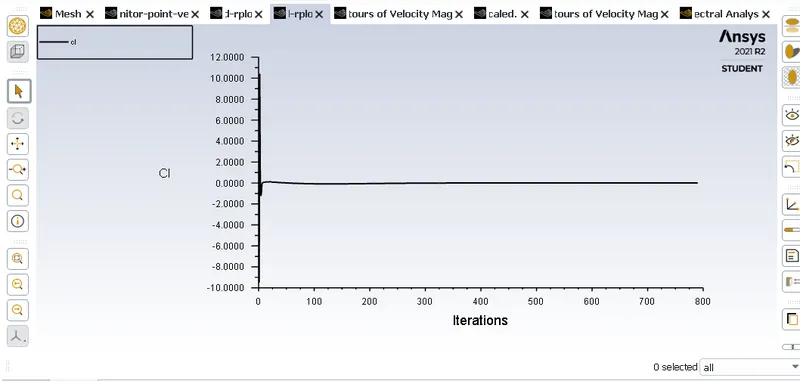
Results for steady state simulation for re = 100
Residual plot
Vertex average of velocity magnitude
Velocity contour
Coefficient of drag plot
Coefficient of lift
Results for steady state simulation for re = 1000
Residual plot
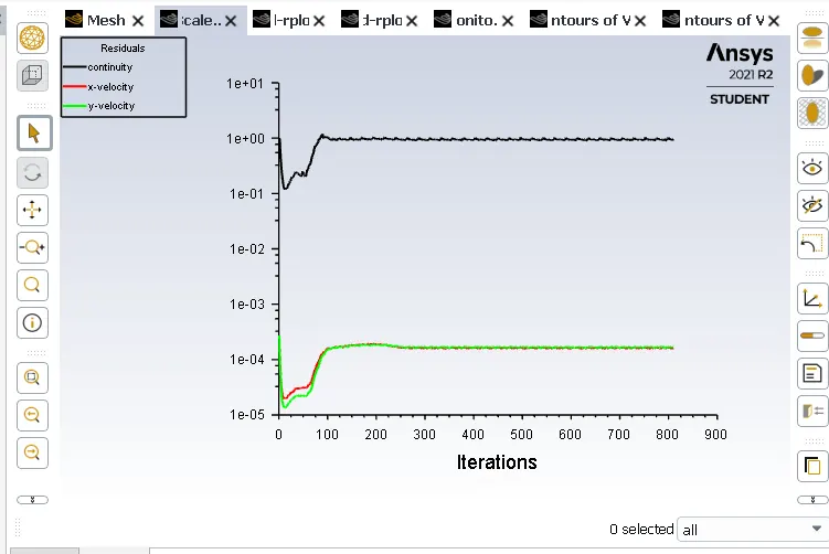
Vertex average of velocity magnitude
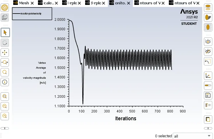
Velocity contour
Coefficient of drag plot
Coefficient of lift
Results for steady state simulation for re = 10000
Residual plot
Vertex average of velocity magnitude
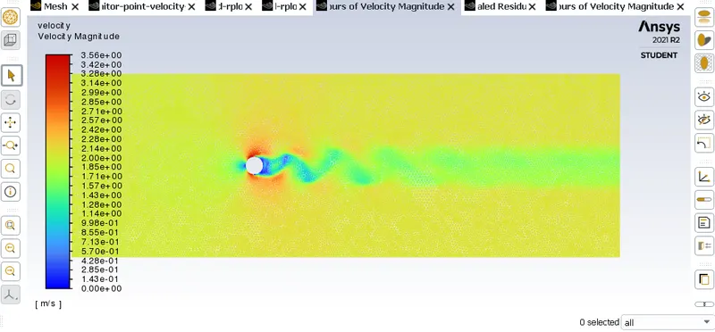
Velocity contour
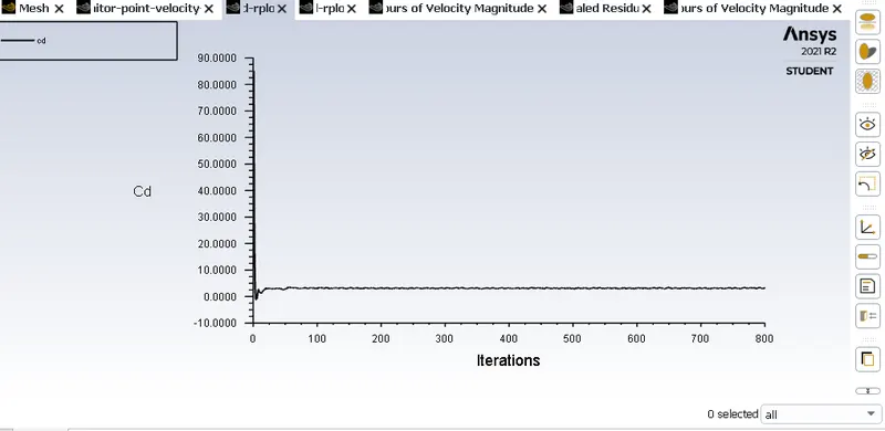
Coefficient of drag plot
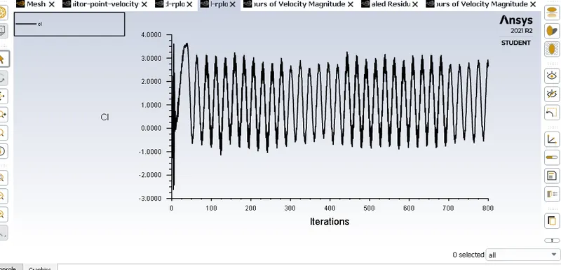
Coefficient of lift
Results for steady state simulation for re = 100000
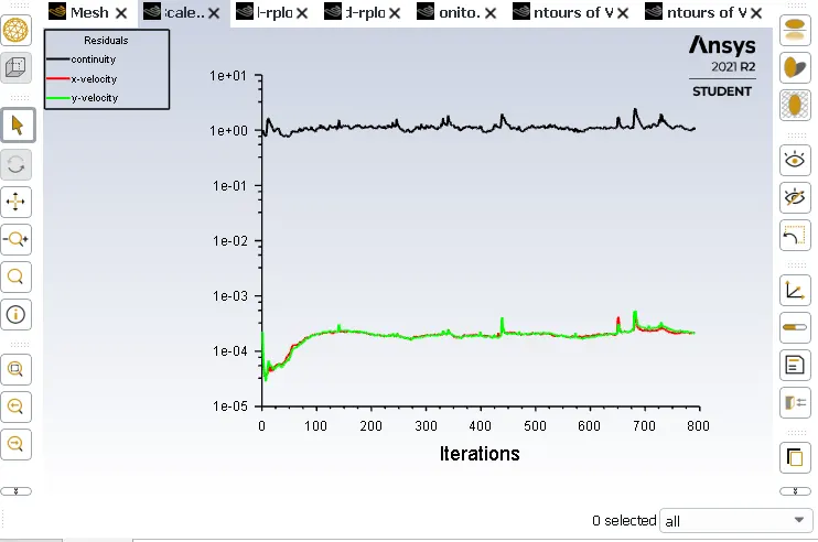
Residual plot
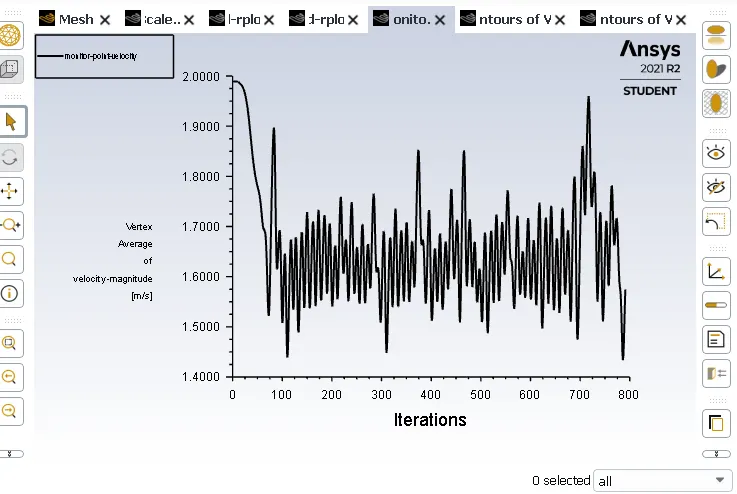
Vertex average of velocity magnitude
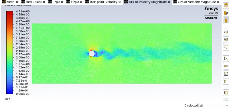
Velocity contour
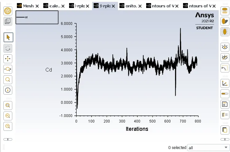
Coefficient of drag plot
Coefficient of lift
Comparison of Reynolds number with Coeffcient of Drag and lift:-
| Reynolds number | Coefficient of Drag | Coefficient of Lift |
| 10 | 3.34 | 0.0011 |
| 100 | 1.68 | 0.048 |
| 1000 | 0.93 | 0.433 |
| 10000 | 0.79 | 0.523 |
| 100000 | 0.825 | 0.678 |
Conclusion :-
- From the above data we can say that simulation get converged with increase in reynolds number effciently.
- From this data we can conclude that the drag coefficient decreases with the Reynolds number increases, and it becomes almost a constant (CD = 0.4) for a Reynolds number between 103 and 2×10⁵. As the Reynolds number increases (Re > 2×10⁵), the boundary layer becomes thinner in the front of the sphere and begins its transition to turbulent. For turbulent boundary layer flow, the drag coefficient is decreased further (e.g., CD = 0.06 for Re = 4×10⁵).
- As the reynolds number increases the wake region behind the cylinder is also increasing which is result in the perfect capturasation of the fluid domain.
- At the low reynolds number (Re<0.4) there is no vortex formation taking place So, we have to increase the reynolds number to see the vonn karman vortex streets flow pattern.
- From this data we can also conclude that the Lift coefficient decreases rapidly and drag coefficient increases rapidly when Reynolds number is decreased below critical range.