Week 2 - Flow over a Cylinder.

OBJECTIVE:

To perform the simulation for flow over a cylinder and investigate the following:

1. Simulate the steady as well as an unsteady flow for Reynolds number = 100 and obtain the Strouhal number.

2. Perform the simulation for Reynolds number = 10, 100, 1000, 10000, & 100000 and calculate the coefficient of drag and lift and discuss the effect of Reynolds number on the coefficient of drag.

SOLUTION:

Introduction:

In real-life engineering, most of the structures consist of the bluff body e.g. high-rise buildings, bridges, cars, aircraft, etc. Whenever flow over a bluff body takes place, it shows a phenomenon of flow separation and vortex shedding in the wake region. At low Reynolds number, this unsteady flow shows a periodic nature of fluctuations in the wake region. This periodic fluctuating force that acts over the structure may lead to the collapse of the structure if the frequency of fluctuating force matches the natural frequency of the structure. So to understand this complex behavior of the fluid in the wake region, the cylinder provides a good model to study.

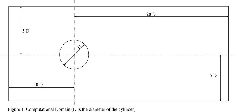
To begin the simulation first we have to consider a computational domain of sufficient size so that the simulation will capture the flow physics accurately. Figure 1, shows the schematic diagram of the computational suggested for this simulation.

Step 1: Creation of geometry in SpaceClaim.

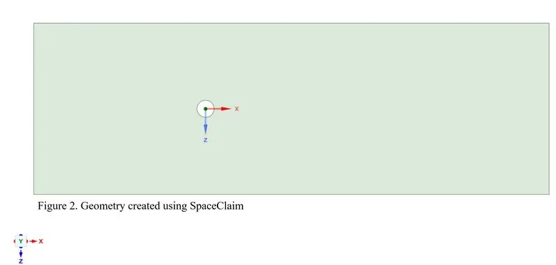
The geometry is being created in created using the various tools available in the interface. Once the raw geometry is created the "PULL" option is being used to convert the geometry into a surface. After that "SELECT" option is being used the surface encircled inside the cylinder wall and then "DELETE" to get the required computational domain. Figure 2, shows the geometry that is being created using the SpaceClaim,

Step 2. Mesh Generation:

Mesh is being created by the following procedure.

Start with MESH >> INSERT >> METHOD and then the parameter is selected whose snippet is shown in fig. 3(a), and the element size is taken as 0.25 m

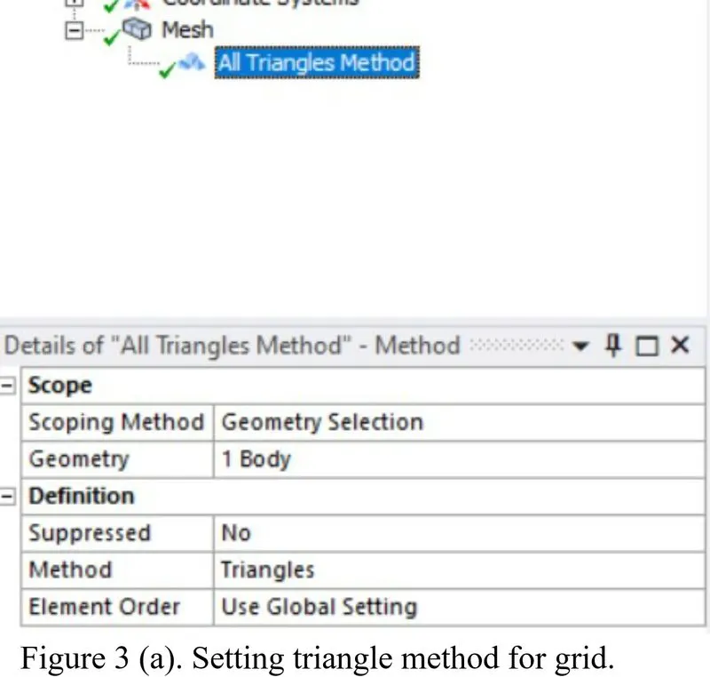
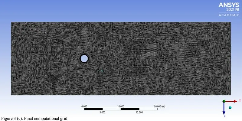
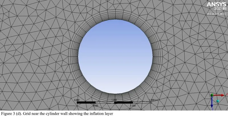
As after adding the TRIANGLES method the grid near the cylinder wall is not refined to capture the variation properly. So near the cylinder wall, the body-fitted grid is required.

GRID >> INSERT >> INFLATION, for the present study 10 layers is being taken,

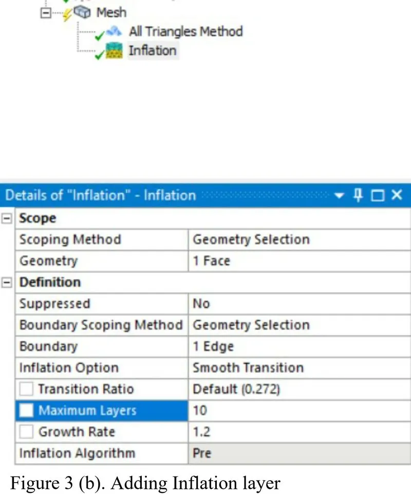
Even after this the grid near the wall is not sufficiently refined so follow GRID >> INSERT >> SIZING, then choose the cylinder wall and divide it into 36 divisions. The final grid and the grid near the wall are shown in fig. 3 (c) and 3 (d) respectively.

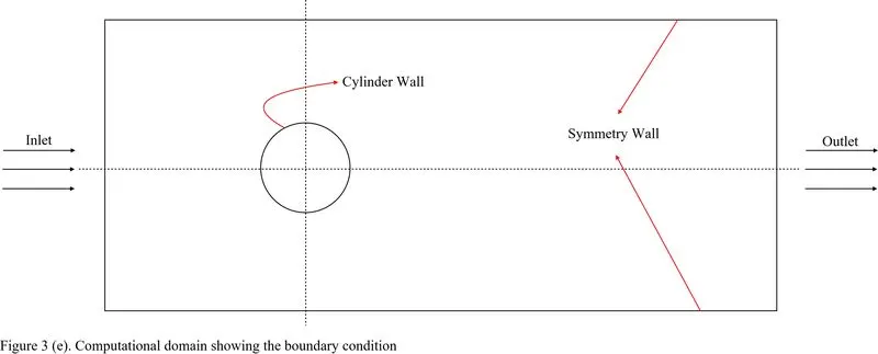
Once the grid is being generated, then name the boundaries which help in specifying the boundary condition while setting up the flow physics. A schematic diagram of the computational domain and the name of the boundary is shown in figure 3 (e).

Step 4. Setting up the flow physics and solution:

CASE 1: Steady flow with Reynolds number = 100

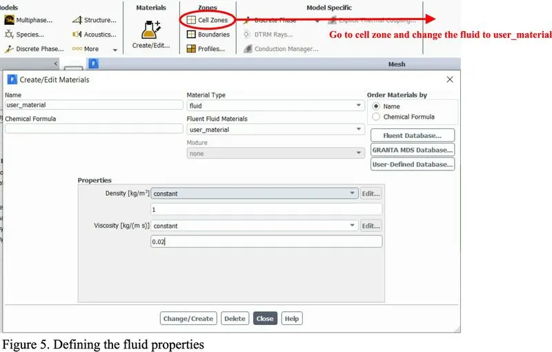
As the Reynolds number is low so we can consider the flow to be laminar and solve the problem considering the laminar model. As we have fixed the Reynolds number first and from it the inlet velocity is being calculated so just for the sake of simplicity the either define a new fluid or change the present property of air as

Density = 1 and the dynamic viscosity as 0.02, as shown in fig 5.

Now define the boundary condition:

At inlet: Velocity inlet boundary condition with velocity = 1 m/s,

While at the outlet, the cylinder wall and the symmetry walls (Refer to figure 3 (e)) were left with default boundary conditions.

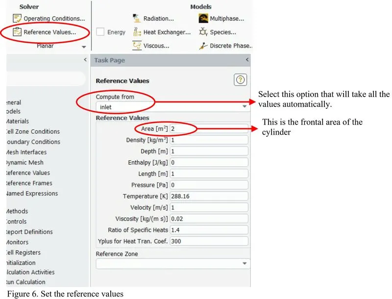
Set the reference values which is required in the calculation of the coefficient of drag and lift. The snippet for the same is shown in figure 6.

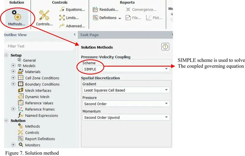
To solve the present problem SIMPLE scheme is used. Snippet of the same is shown in figure 7.

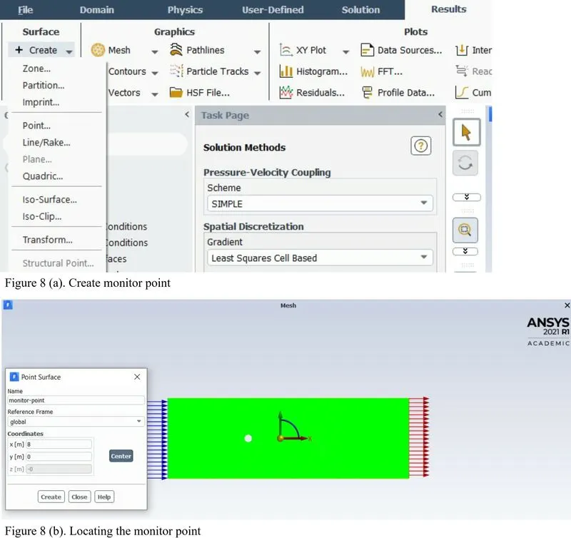
Now go to DEFINITION to calculate and take the plot of the coefficient of drag and lift and the velocity at a monitor point located at "4D" downstream along the centreline. So first there is a need to create a monitor point. To create the monitor point "RESULTS >> SURFACE >> CREATE >> POINT"

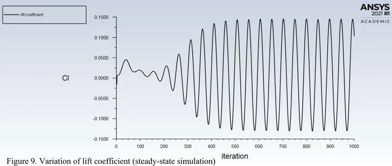
Now initialize the variables and specify the number of iteration for solving the problem. For the present problem, simulation is performed for 1000 iteration.

So plots obtained for the steady-state simulation are as follows:

Case 2. Unsteady-flow with Reynolds number = 100

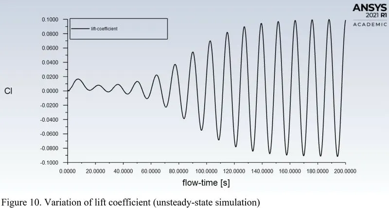
To perform the transient simulation everything will be the same only at the start "TRANSIENT" model is to be selected and time steps is to be specified, for the present simulation time step is taken as 0.2 sec. Also instead of a number of iteration, the number of time steps is specified, for the present case simulation is performed for 1000 time steps i.e. the flow time is 200 sec.

Strouhal number:

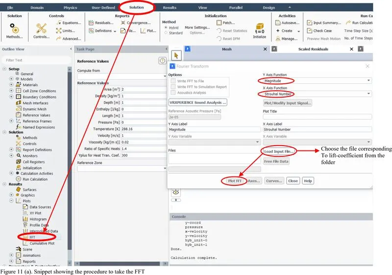
This is a dimensionless number used to describe the vortex shedding frequency for an unsteady oscillating flow. Now to compute the strouhal number in ANSYS FLUENT, FFT (Fast Fourier Transform) of the data containing the fluctuation of the coefficient of lift is taken, and then exporting the data file generated after taking the FFT in an excel file. The value corresponding to the maximum magnitude is the Strouhal number.

The same is being shown through the snippet in figure 11.

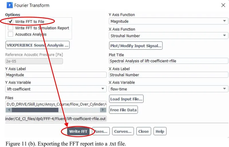
So, for the present study, the strouhal number computed is found to be 0.1598. The same is being validated from paper [1].

Comparison of drag coefficient for different Reynolds numbers:

Steady-state simulation is performed by following the same procedure as discussed above for Reynolds numbers `10, 10^2, 10^3, 10^4, & 10^5`. To change the Reynolds number only the velocity at the inlet is kept on changing while the other parameters like density and viscosity are kept constant. (Note: For Reynolds number `10^4 & 10^5` `k-epsilon` turbulence model is being used).

Following plots are obtained:

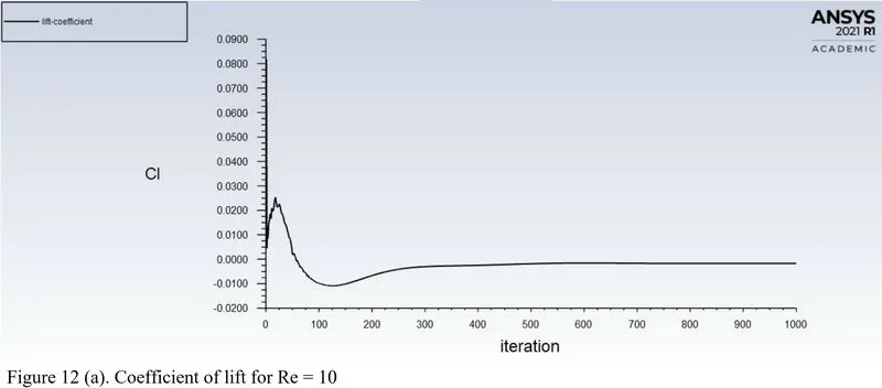
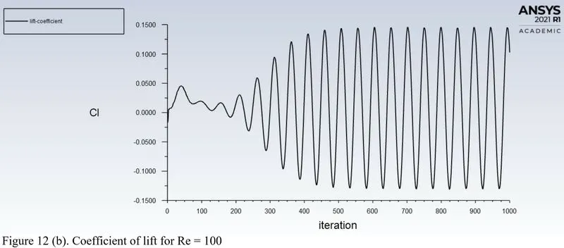
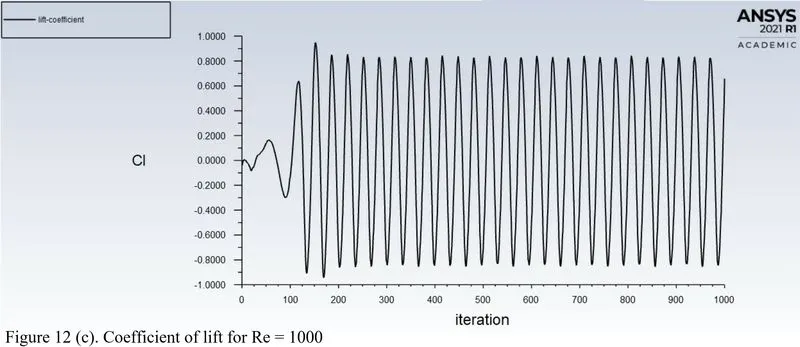
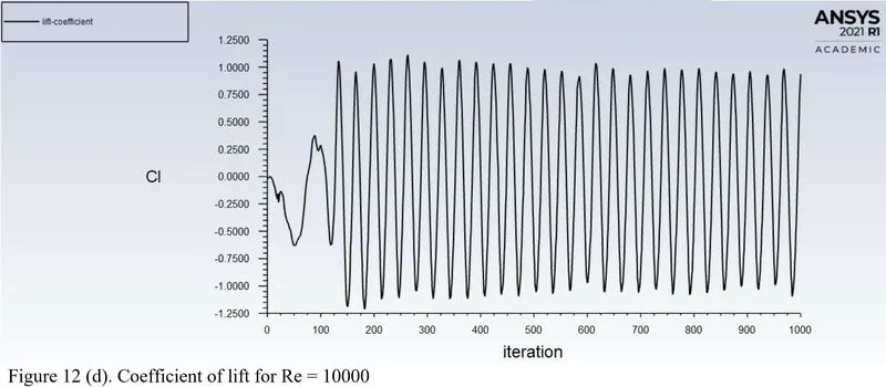
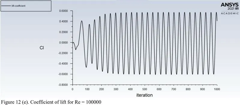
Coefficient of Lift:

Velocity at the monitor point:

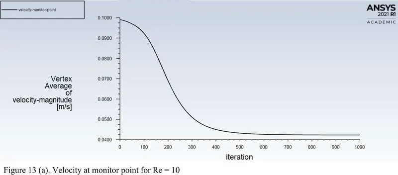
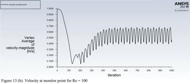
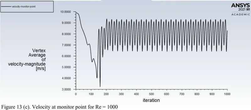
To see the vortex shedding effect a monitor point is being created and the velocity at that point is plotted. The monitor point created is shown in figure 8(b).

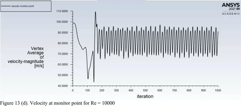
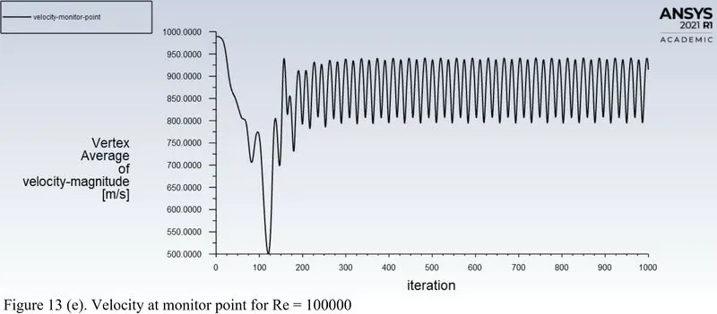
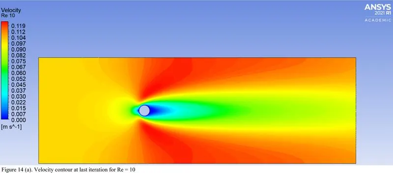
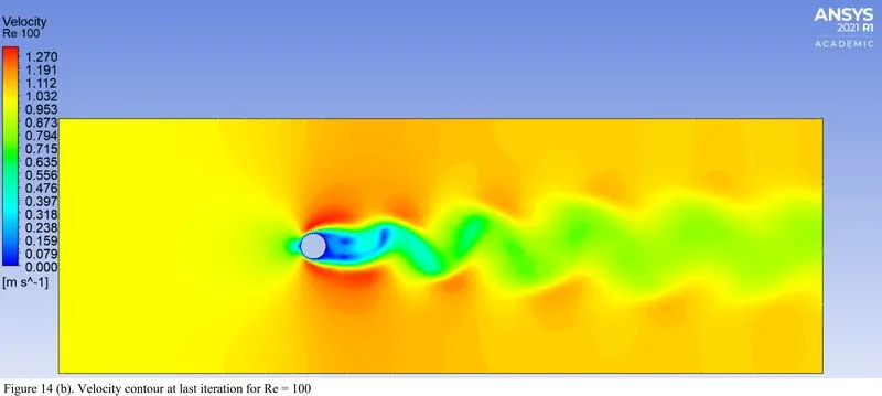
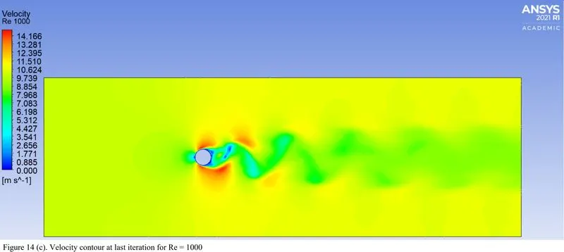
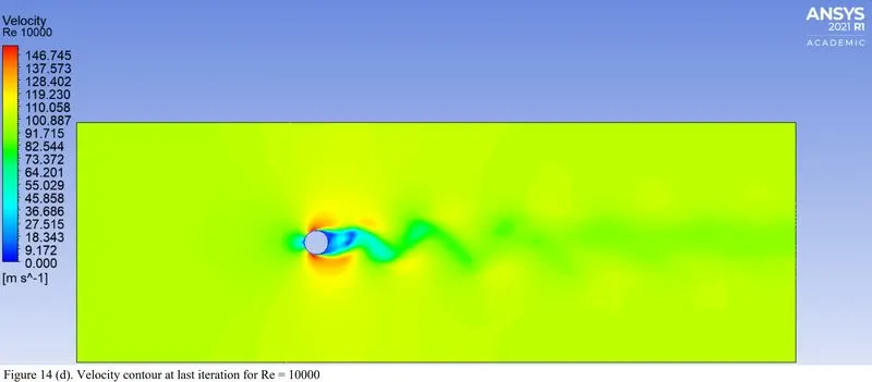
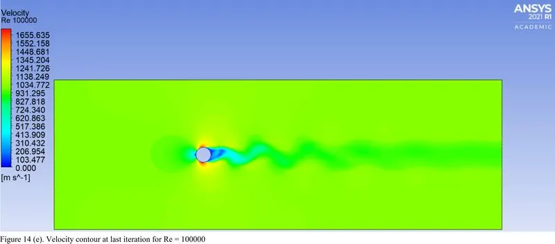
Velocity contours at the last iteration:

Velocity contour is obtained for the last iteration for the range of Reynolds number.

Results:

The mean drag and lift coefficient is being calculated from the report file generated for the same. Convert that report file into .txt file and then export that file into MS-Excel from where the mean of the data is being calculated. The obtained value is being tabulated as shown in table 1.

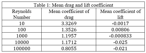
From the above table, the lift coefficient seems to approxixmately equal to zero which is correct according to the flow physics because the cylinder is placed at symmetrically with respect to the flow direction.

Conclusion:

1. There is no vortex shedding phenomenon is being observed at Reynolds number = 10. [Refer figure 13(a) and 14(a)]

2. As the Reynolds number is increased there is reduction in the mean value of coefficient of drag.

References:

1. Control of laminar vortex shedding behind a circular cylinder using splitter plates, Kiyoung Kwon & Haecheon Choi, Physics of fluids, 1996.