Week - 2 - Explicit and Implicit Analysis

Explicit and Implicit Analysis

1.Aim: To differntiate between Implicit and Explicit Analyses by solving the equation `f(u)=u^3+9u^2+4u` using both Implicit and Explicit methods to a tolerance of 0.01.

2.Objective: 

1. To explain the difference between Implicit and Explicit Analyses.
2. To solve the given function `f(u)=u^3+9u^2+4u` using both Implicit and Explicit Methods.
3. To plot the graphs for the above function for both Implicit and Explicit methods.

3. Solving the eqn `f(u)=u^3+9u^2+4u` using Implicit and Explicit Methods:

Given eqn is `f(u)=u^3+9u^2+4u` which represents the internal resisting force upon application of an external load "F".
Let "k"=Stiffness
      "u"=Displacement
      "`Deltau`" and "`DeltaF`"be incremental displacement and Load(externally applied) respectively.

Let us assume that the Total Load "F" is applied in 3 equal load increments each equals to `DeltaF=1`
We will be making use of the eqn ∆F = k∆u
From this, ∆u=∆F/k;  `k(u)=(df)/(du`
That is, `k(u)=3u^2+18u+4`

Hence, we have `f(u)=u^3+9u^2+4u` and `k(u)=3u^2+18u+4`........(i)

Explicit Method:

Step1: Let initial displacement `u_underset(0)`=0
`k[u]_underset(0).Deltau_underset(1)`=`DeltaF_underset1`
`implies``k[0].Deltau_underset(1)`=`DeltaF_underset1`
`implies``Deltau_underset(1)=(DeltaF)/(k[u]_underset(0)`
`implies``Deltau_underset(1)=1/4=0.25`

Now, u₁= u₀+`Delta`u₁  `implies` u₁=0.25
f(u₁)=f(0.25)= `0.25^3+(9**0.25^2)+(4**0.25)`=1.578125;   f(u₁)=1.578125

R₁=|F₁-f(u₁)|=|1-1.578125|
R₁=0.578125

k(u₁)=k(0.25)=(3*0.25²)+(18*0.25)+4 `implies` k(u₁)=8.6875

Step2: 
`k[u]_underset(1).Deltau_underset(2)`=`DeltaF_underset2`
`implies``k[0.25].Deltau_underset(2)`=`DeltaF_underset2`
`implies``Deltau_underset(2)=(DeltaF)/(k[u]_underset(1)`
`implies``Deltau_underset(2)=1/8.6875=0.11511`

Now, u₂= u₁+`Delta`u₂  `implies` u₂=0.36511
f(u₂)=f(0.36511)= `0.36511^3+(9**0.36511^2)+(4**0.36511)`=2.70886;   f(u₂)=2.70886

R₂=|F₂-f(u₂)|=|2-2.70886|
R₂=0.70886

k(u₂)=k(0.36511)=(3*0.36511²)+(18*0.36511)+4 `implies` k(u₂)=10.97190

Step3: 
`k[u]_underset(2).Deltau_underset(3)`=`DeltaF_underset3`
`implies``k[0.36511].Deltau_underset(3)`=`DeltaF_underset3`
`implies``Deltau_underset(3)=(DeltaF)/(k[u]_underset(2)`
`implies``Deltau_underset(3)=1/10.97190=0.09114`

Now, u₃= u₂+`Delta`u₃  `implies` u₃=0.45625
f(u₃)=f(0.45625)= `0.45625^3+(9**0.45625^2)+(4**0.45625)`=3.79345;   f(u₃)=3.79345

R₃=|F₃-f(u₃)|=|3-3.79345|
R₃=0.79345

k(u₃)=k(0.45625)=(3*0.45625²)+(18*0.45625)+4 `implies` k(u₃)=12.83699

Stepi	`Delta`Fi	`Delta`ui	ui	(Fext) i	(fint)i	fint-Fext=R
1	1	0.25	0.25	1	1.57813	0.57813
2	1	0.11511	0.36511	2	2.70886	0.70886
3	1	0.09114	0.45625	3	3.79345	0.79345

Implicit Method:

• An implicit analysis is the same as the explicit analysis, except that at the end of each step Newton-Raphson iterations are used to enforce equilibrium before moving to the next step.
• Basically, an incremental force is applied to advance the solution forward at the beginning of a step.
• However, internal forces and external forces will not be in equilibrium unless the stiffness is linear for the given step.
• Hence, in order to achieve equilibrium, corrections must be made to the displacement.
• This is accomplished by using Newton-Raphson iterations to minimize the residual, R(u) = f_int − F_ext
• Expanding the residual as a Taylor series about the current displacement u^j gives 
  
  R^j+1 = R^j(u^j)+ [dR(u^j) /du] *δu^j+1 +... = R^j +k(u^j)δu^j+1 +………..... (ii) 
  
  By neglecting higher order terms in the series, setting R^j+1 = 0  and solving for δu^j+1  the following correction is obtained 
  

  
  δu^j+1 = −[k(u^j)]⁻¹R^j ..................(iii)
  
  

• Notice that the iteration variable is "j" and it may take several iterations for the norm of the residual, ||R||, to be reduced below the chosen tolerance criteria, i.e, 0.01 

Step1: Let initial displacement `u_underset(0)`=0
`k[u]_underset(0).Deltau_underset(1)`=`DeltaF_underset1`
`implies``k[0].Deltau_underset(1)`=`DeltaF_underset1`
`implies``Deltau_underset(1)=(DeltaF)/(k[u]_underset(0)`
`implies``Deltau_underset(1)=1/4=0.25`

Now, u₁= u₀+`Delta`u₁  `implies` u⁽⁰⁾₁=0.25

f(u⁽⁰⁾₁)=f(0.25)= `0.25^3+(9**0.25^2)+(4**0.25)`=1.578125;  f(u⁽⁰⁾₁)=1.578125

R⁽⁰⁾₁=|F₁-f(u⁽⁰⁾₁)|=|1-1.578125|
R⁽⁰⁾₁=0.578125 > 0.01

Therefore, Newton-Raphson iterations are required.

Iteration 01:
k(u⁽⁰⁾₁)=k(0.25)=(3*0.25²)+(18*0.25)+4 `implies` k(u⁽⁰⁾₁)=8.6875

From (iii),
δu^j+1 = −[k(u^j)]⁻¹R^j
`implies`δu₁⁽¹⁾ = −[k(u₁⁽⁰⁾)]⁻¹R₁^{(0)
`implies`}δu₁⁽¹⁾ = −[8.6875]⁻¹ x 0.578125
^`implies`δu₁⁽¹⁾ = -0.06655

u₁⁽¹⁾= u₁⁽⁰⁾+`delta`u₁⁽¹⁾  `implies` u₁⁽¹⁾=0.25-0.06655
`implies` u₁⁽¹⁾=0.18345

f(u⁽¹⁾₁)=f(0.18345)= `0.18345^3+(9**0.18345^2)+(4**0.18345)`=1.04286;  f(u⁽¹⁾₁)=1.04286

R⁽¹⁾₁=|F₁-f(u⁽¹⁾₁)|=|1-1.04286|
R⁽¹⁾₁=0.04286 > 0.01

Iteration 02:
k(u⁽¹⁾₁)=k(0.18345)=(3*0.18345²)+(18*0.18345)+4 `implies` k(u⁽¹⁾₁)=7.40306

Therefore,   δu₁⁽²⁾ = δu₁⁽¹⁾−[k(u₁⁽¹⁾)]⁻¹R₁⁽¹⁾

^`implies`δu₁⁽²⁾ = -0.06655−[7.40306]⁻¹ x 0.04286

^`implies`δu₁⁽²⁾ = -0.07234

u₁⁽²⁾= u₁⁽⁰⁾+`delta`u₁⁽²⁾  `implies` u₁⁽²⁾=0.25-0.07234
`implies` u₁⁽²⁾=0.17766

f(u⁽²⁾₁)=f(0.17766)= `0.17766^3+(9**0.17766^2)+(4**0.17766)`=1.000315;  f(u⁽²⁾₁)=1.00032

R⁽²⁾₁=|F₁-f(u⁽²⁾₁)|=|1-1.00032|
R⁽²⁾₁=0.00032 < 0.01

k(u⁽²⁾₁)=k(0.17766)=(3*0.17766²)+(18*0.17766)+4 `implies` k(u⁽²⁾₁)=7.29257


Step2: 
k[u⁽²⁾₁].`Delta`u⁽⁰⁾₂=`DeltaF_underset2`
`implies`k[0.17766].`Delta`u⁽⁰⁾₂=`DeltaF_underset2`
`implies``Delta`u⁽⁰⁾₂=`DeltaF`/k[u⁽²⁾₁]
`implies``Delta`u⁽⁰⁾₂=1/7.29257=0.13713
`implies``Delta`u⁽⁰⁾₂=0.13713

Now, u⁽⁰⁾₂= u⁽²⁾₁+`Delta`u⁽⁰⁾₂  `implies` u⁽⁰⁾₂=0.31479

f(u⁽⁰⁾₂)=f(0.31479)= `0.31479^3+(9**0.31479^2)+(4**0.31479)`=2.18219;  f(u⁽⁰⁾₂)=2.18219

R⁽⁰⁾₂=|F₂-f(u⁽⁰⁾₂)|=|2-2.18219|
R⁽⁰⁾₂=0.18219 > 0.01

Therefore, Newton-Raphson iterations are required.

Iteration 01:
k(u⁽⁰⁾₂)=k(0.31479)=(3*0.31479²)+(18*0.31479)+4 `implies` k(u⁽⁰⁾₂)=9.96350

From (iii),
δu^j+1 = −[k(u^j)]⁻¹R^j
`implies`δu₂⁽¹⁾ = −[k(u₂⁽⁰⁾)]⁻¹R₂^{(0)
`implies`}δu₂⁽¹⁾ = −[9.96350]⁻¹ x 0.18219
^`implies`δu₂⁽¹⁾ = -0.01829

u₂⁽¹⁾= u₂⁽⁰⁾+`delta`u₂⁽¹⁾  `implies` u₂⁽¹⁾=0.31479-0.01829
`implies` u₂⁽¹⁾=0.2965

f(u⁽¹⁾₂)=f(0.2965)= `0.29655^3+(9**0.2965^2)+(4**0.2965)`=2.00328;  f(u⁽¹⁾₂)=2.00328

R⁽¹⁾₂=|F₂-f(u⁽¹⁾₂)|=|2-2.00328|
R⁽¹⁾₂=0.00328 < 0.01

No further iterations are required.

k(u⁽¹⁾₂)=k(0.2965)=(3*0.2965²)+(18*0.2965)+4 `implies` k(u⁽¹⁾₂)=9.60074

Step3: 
k[u⁽¹⁾₂].`Delta`u⁽⁰⁾₃=`DeltaF_underset3`
`implies`k[0.2965].`Delta`u⁽⁰⁾₃=`DeltaF_underset3`
`implies``Delta`u⁽⁰⁾₃=`DeltaF`/k[u⁽¹⁾₂]
`implies``Delta`u⁽⁰⁾₃=1/9.60074=0.10416
`implies``Delta`u⁽⁰⁾₃=0.10416

Now, u⁽⁰⁾₃= u⁽¹⁾₂+`Delta`u⁽⁰⁾₃  `implies` u⁽⁰⁾₃=0.40066

f(u⁽⁰⁾₃)=f(0.40066)= `0.40066^3+(9**0.40066^2)+(4**0.40066)`=3.11171;  f(u⁽⁰⁾₃)=3.11171

R⁽⁰⁾₃=|F₃-f(u⁽⁰⁾₃)|=|3-3.11171|
R⁽⁰⁾₂=0.11171 > 0.01

Therefore, Newton-Raphson iterations are required.

Iteration 01:
k(u⁽⁰⁾₃)=k(0.40066)=(3*0.40066²)+(18*0.40066)+4 `implies` k(u⁽⁰⁾₃)=11.69347

From (iii),
δu^j+1 = −[k(u^j)]⁻¹R^j
`implies`δu₃⁽¹⁾ = −[k(u₃⁽⁰⁾)]⁻¹R₃^{(0)
`implies`}δu₃⁽¹⁾ = −[11.69347]⁻¹ x 0.11171
^`implies`δu₃⁽¹⁾ = -0.00955

u₃⁽¹⁾= u₃⁽⁰⁾+`delta`u₃⁽¹⁾  `implies` u₃⁽¹⁾=0.40066-0.00955
`implies` u₃⁽¹⁾=0.39111

f(u⁽¹⁾₃)=f(0.39111)= `0.39111^3+(9**0.39111^2)+(4**0.39111)`=3.00097;  f(u⁽¹⁾₂)=3.00097

R⁽¹⁾₃=|F₃-f(u⁽¹⁾₃)|=|3-3.00097|
R⁽¹⁾₃=0.00097 < 0.01

No further iterations are required.

Stepi	`Delta`Fi	ui	(Fext) i	(fint)i	fint-Fext=R
1	1	0.17766	1	1.00032	0.00032
2	1	0.29650	2	2.00328	0.00328
3	1	0.39111	3	3.00097	0.00097

 4.Plots:

i.Explicit Analysis: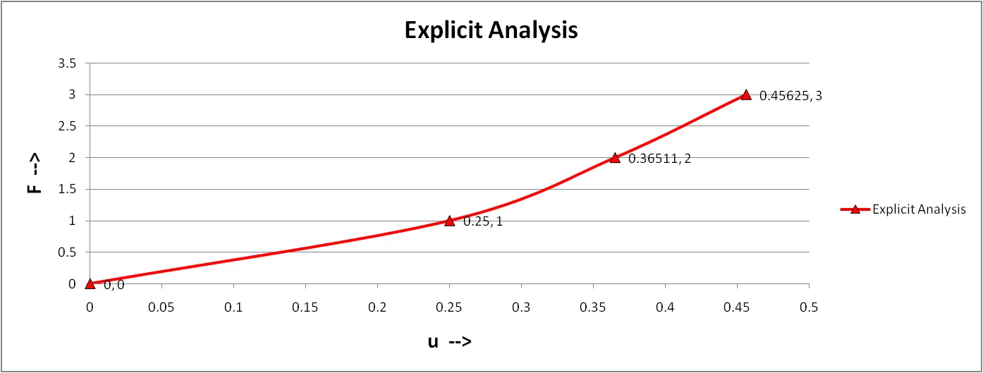



ii.Implicit Analysis: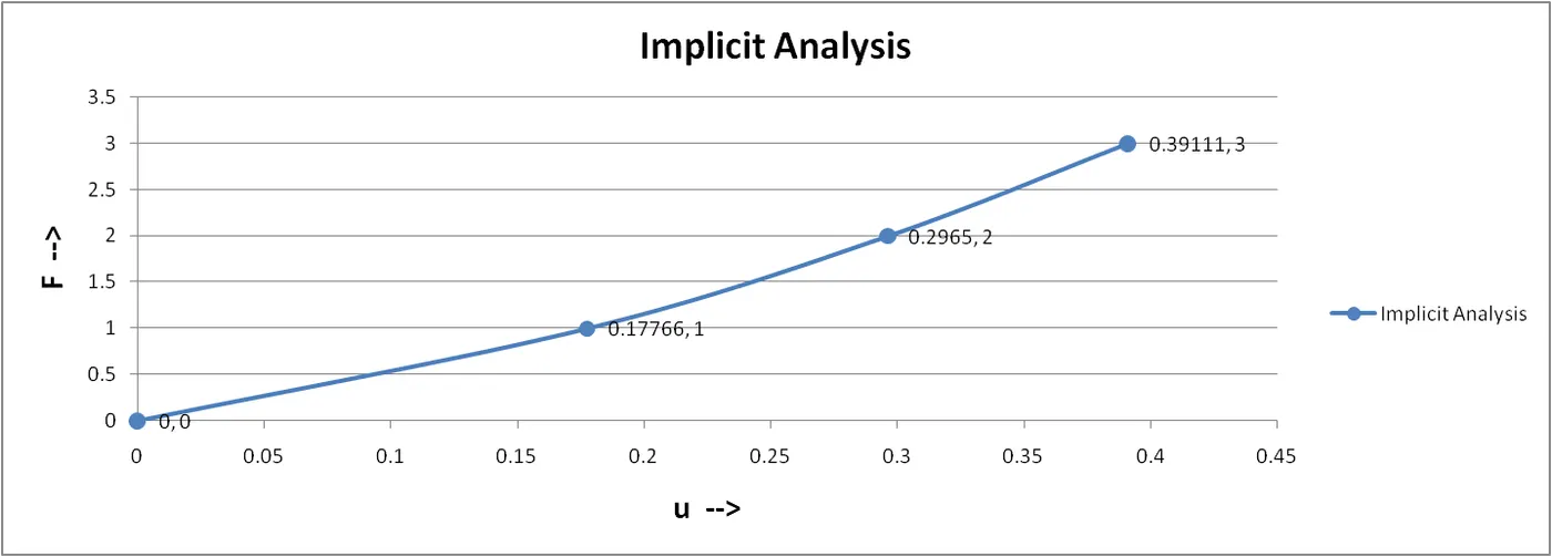



iii.Explicit vs Implicit Analysis: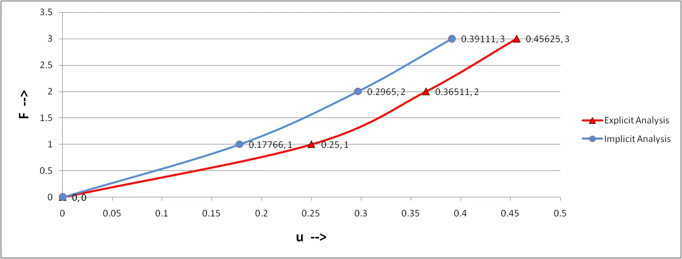

• It is evident from the plot that the explicit analysis drifts from the exact solution.  
• The drift from the exact solution illustrates the lack of equilibrium between the internal and external forces.
• To correct for this problem an implicit analysis is required.
• The Newton-Raphson iterations correct the incremental steps so that they land on the exact solution according to the specified tolerance. Excellent agreement is achieved with just 3 increments and in each step only two Newton-Raphson iterations are required. 

5. Explicit vs Implicit Analysis:

Both Implicit and Explicit Analysis are used to solve Partial Differential Equations (PDE's). Both techniques are valid methods for solving time-dependent problems but there are differences between them that help explain why different kinds of methods are suited to each methods.

Implicit FEA:

Implicit FEA is a numerical technique to solve differential equations by discretizing them into a system of algebraic equations that can be solved using matrix methods. In Implicit FEA, the state of component is defined as a function of present and future states.

Implicit FEA is best suited for analyzing static or low speed phenomena and the solution is calculated for large time steps.

Eg of Implicit Analysis:
i. Low Frequency Response
ii. Vibrations
iii. Oscillations

Explicit FEA:

In Explicit FEA, also known as dynamic analysis, the analyst applies loads to the model and lets the software compute deformation, stress and strain. This method is best suited for highly non-linear problems or problems with complex contact conditions. Explicit FEA calculation is done with a very small time step of 10^-6 seconds.

For eg, if an engineer needs to know how much force it would take for someone to break through a wall, they need to use explicit FEA software.

Some Analysis utilising Explicit method include:
i.Car Crash
ii.Drop Test
iii.Impact
iv.Blast
v.FSi(Flow Structure index)

Explicit	Implicit
1. No Iterations	1. Iterations required for Non-Linear problem
2. Conditionally stable, Courant-Friedrich-Levy (CFL) criteria	2. Unconditionally stable
3. Needs low memory	3. Higher memory
4. Relatively smaller timesteps	4. Large timesteps and may change due to non-linearities
5. Spatial derivative evaluated at ‘n’ time intervals [Mn]{`ddot u`n}+[Cn]{`dot u`n}+[kn]{un}={Fn}	5. Spatial derivative evaluated at ‘n+1’ time intervals [Mn+1]{`ddot u`n+1}+[Cn+1]{`dot u`n+1}+[kn+1]{un+1}={Fn+1}

Explanation:

1.Iterations:

Let us consider an eqn u^(t+1)=u^t+u'`Deltat` `implies` u^(t+1)=u^t+`(du)/dt`.`Deltat`

Here if `((du)/dt)^t``implies`Explicit Analysis since now u^(t+1)=u^t+`((du)/dt)^t``Deltat`   has RHS all known values in terms of time interval 't'. Therefor no iteration are required.

And if `((du)/dt)^(t+1)``implies`Implicit Analysis since now u^(t+1)=u^t+`((du)/dt)^(t+1)``Deltat`  has unknown values in both LHS and RHS in terms of time interval 't+1'. Hence Implicit Analysis needs iterations.

We know that the basic governing equation in FEA is
[M]{`ddot u`}+[C]{`dot u`}+[k]{u}={R} which in static reduces to [k]{u}={R} where R=|f(u)-F| in which f(u) represents internal force and F externally applied load. While doing analysis by explicit method even if R is not in euilibrium(say within a tolerance of 10^-5) in a particular step, we will still move on to the next Timestep.

But in Implicit Analysis we won't move onto the next step until and unless we achieve in required tolerance in current step. For this we use Newton- Raphson Iterations [as explained in detail in section 3 of this report]

2.Stability:

i. Each timestep in Explicit Analysis is verfy fast but it works only when timestep `Delta T`is very small. To determine the size of timestep, we have a criteria called Courant Friedrich Levy's(CFL) criteria which dictates that the timestep must be smaller than elastic wave to propagate from one side of element to other.

`DeltaT=Lsqrt((rho(1-2nu))/(2mu(1-nu)`=`(Lc)/C`

where 'Lc' represents the characteristic length of element and 'C' represents the speed of sound or elatic wave in the element.

If `DeltaT`is too small computational time increases and length of element decreases. If its too large it won't satisfy the criteria. Hence, `DeltaT` should have optimal value to satisfy CFL criteria to achieve stabe solution.
Therefore, Explicit Analysis is called Conditionally Stable.

ii. In case of Implicit Analysis, there is timestep but it is Pseudo Timestep which means Timestep is an indirect way of dividing the Load into steps inorder to achieve convergence.

eg: Assume F=100kN. If we apply 100kN at once it might give convergence issue, so to avoid this we can use substeps. This can be done by using Timesteps.

Let 100kN is to be applied in 1sec, say we are using a timestep of 0.1 sec. Then there would be 10 timesteps.

Considering these 10 timesteps each Loadstep would be 10kN. Hence, we have divided the total load into substeps as per the chosen timesteps to achieve convergence.

Since there is no such criteria to determine the timestep to achieve stability, Implicit Analysis is unconditionally stable.

3.Memory requirement:

Implicit Analysis requires more memory when compared to Explicit Analysis.

Explicit Analysis:

We know, 
[M]{`ddot u`}+[C]{`dot u`}+[k]{u}={R} `implies`Acceleration {`ddot u`}=[M]^-1[{R}-[C]{`dot u`}+[k]{u}]. Upon double integrating this we get Nodal displacement matrix {u}
Here Nodal Mass Matrix, [M] is symmetric as well as diagonal. Hence, inverting it is easy and requires less memory.

Implicit Analysis:

[K][`Deltau`]ⁱ=[R]ⁱ `implies`[`Deltau`]ⁱ=[K]^-1Rⁱ

Here stiffness matrix [K] is symmetric but not diagonal. Hence, inverting it requires high memory. [K]^-1 can be found out by direct or iterative methods.

4.Timestep size:
Self explanatory from section 2 Stability.

5.Spatial Derivative Evaluation:
Spatial Derivative is evaluated at 'n' time intervals for Explicit Analysis and 'n+1' time intervals for Implicit Analyis.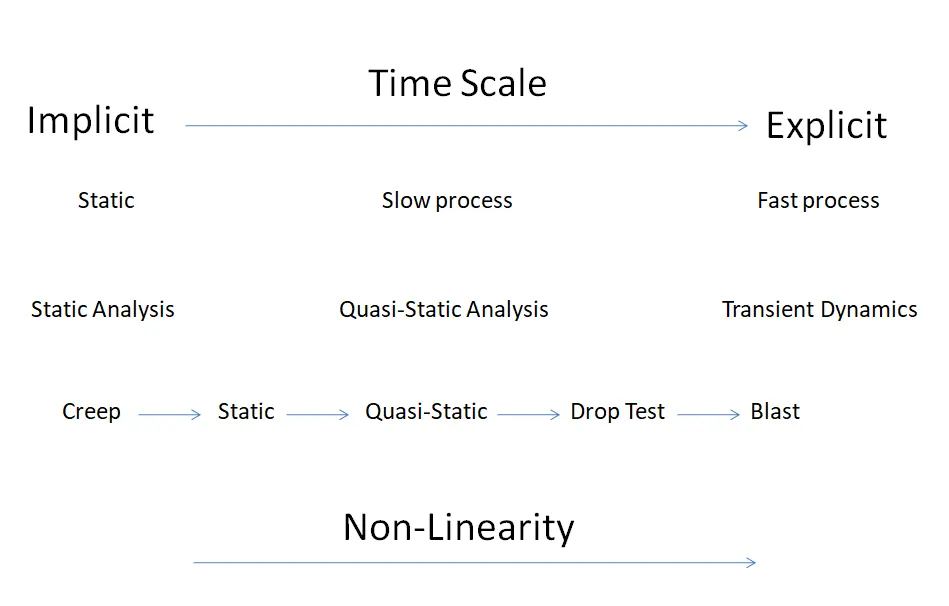

6. Conclusion:

There is no exact answer to which analysis is better: Implicit or Explicit. Both are methods by which we can do different types of analyses but a particular method may be favourable for a particular set of analyses while the other would favour some other types of analyses.

Implicit is a good choice for structure dynamic types of problems for which the load rate is slow. Ideal Analysis typically takes more time than one second. The ability for users to set any time increment is an added advantage.The Stiffness Matrix inversion gives unknown x. Enforced equilibrium solutions for Newton-Raphson.

eg: i.Low Frequency Response
     ii.Vibration
    iii.Oscillation

For quick events, the Explicit solver is excellent(mostly less than 0.1 second). The Explicit solver determines the size of time increment and sets it. The density of the substance affects the speed of sound in the medium. Mass scaling refers to this. The mesh, young's Modulus and density all affect explicit timestep.
eg: Wave Propagation problems like 
i.Car Crash
ii.Drop
iii.Impact
iv.Blast
v.FSi(Flow Structure Index)