Project 1 - Parsing NASA thermodynamic data

Program:Parsing NASA Thermodynamic Data

1.Aim: To write a code in Matlab to parse the NASA thermodynamic data file and use it to evaluate the thermodynamic properties of the given gas species.

2.Objectives:

1. To write a function that extracts the 14 coefficients and to calculate the enthalpy,entopy and specific heats for all the species in the data file using the local temperature ranges of the individual species.
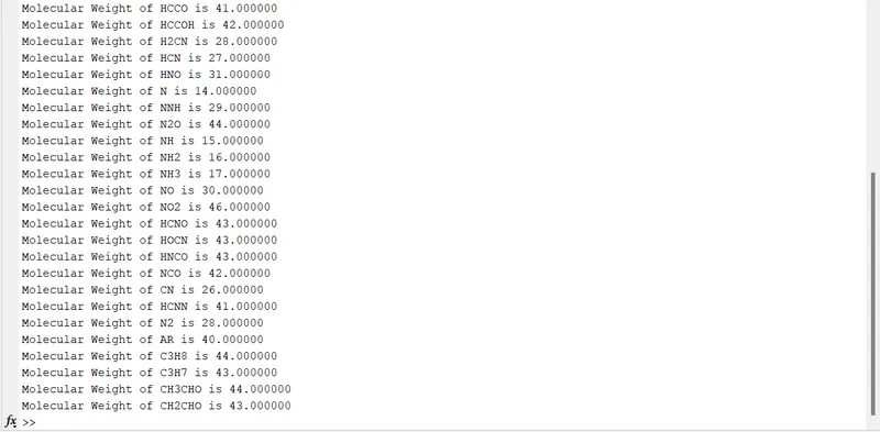
2. To calculate the molecular weight of each species and display it in the command window.
3. To plot the Cp,Enthalpy,Entropy for the local temperature range specific for each species.
4. To automatically save the plots as images with appropriate names and store them in separate folders for each species with the respective species name.

3.Theory:

File Parsing: Parsing a file means reading in a data stream of some sort and building an in memory model of the semantic content of that data. This aims at facilitating perfoming some kind of transformation on the data.In Layman's terms, File Parsing refers to how the information can be read from a particular file and be used in a computer program.

NASA Thermodynamic Data: The NASA Thermodynamic Data is provided to us in the form of a '.dat' file named "THERMO.dat".The file contains information regarding 53 species which includes their Local Temperature Ranges(ranging from low to high) and the corresponding Thermodynamic Coefficients 'a1 a2 a3 a4 a5 a6 a7 a8 a9 a10 a11 a12 a13 a14'. Out of these 14 coefficients, the former 7 coefficients represent the High Temperature Coefficients and the latter 7 represent the Low Temperature Coefficients.Global Temperature Range is also mentioned in the file.

4.Governing Equations: The Polynomial Equations to calculate the Thermodynamic Properties which are used in this program are listed below:

1. Specific Heat at Constant Pressure(Cp): Specific heat is a thermodynamic property, which is defiend as the amount of heat which is required to raise the temperature of a unit mass of substance by one degree celcius.
   `C_p=R*(a_1+a_2*T+a_3*T^2+a_4*T^3+a_5*T^4)` for high local temperature range
   `C_p=R*(a_8+a_9*T+a_10*T^2+a_11*T^3+a_12*T^4)` for low local temperature range
2. Enthapy(H):Enthalpy , a property of a thermodynamic system, is equal to the system's internal energy plus the product of its pressure and volume. For a closed system undergoing a thermodynamic process at constant pressure, the heat absorbed or released equals to the change in enthalpy.
   `H=R*T(a_1+a_2*(T)/2+a_3*T^2/3+a_4*T^3/4+a_5*T^4/5+a_6/T)` for high local temperature range
   `H=R*T(a_8+a_9*(T)/2+a_10*T^2/3+a_11*T^3/4+a_12*T^4/5+a_13/T)` for low local temperature range
3. Entropy(S):In Statistical Thermodynamics, Entropy is defined as the measure of molecular disorderness,i.e., uncertainity in the position of molecule at any instant of time.The term, Entropy comes into picture upon application of the Second Law of Thermodynamics for a process.Since, entropy is a thermodynamic property, it has a unique value at a defined state irrespective of whether the process is reversible or irreversible.
   `S=R*(a_1*lnT+a_2*T+a_3*T^2/2+a_4*T^3/3+a_5*T^4/4+a_7)` for high local temperature range
   `S=R*(a_8*lnT+a_9*T+a_10*T^2/2+a_11*T^3/3+a_12*T^4/4+a_14)` for low local temperature range

Here 'R' represents the 'Universal Gas Constant(8.314 KJ/Kmol.K)' and 'T' represents the 'Local Temperature Range'.

5.Code:

5.1Main Code:

clear all;
close all;
clc;

%Parsing NASA Thermodynamic data and to caluculate Cp,H,S,MW for all the species

%inputs
R=8.314; %where R=Universal gas constant in KJ/kmol.K


%Reading the NASA Thermodynamic Data
f1=fopen('THERMO.dat','r');
fgetl(f1);
Global_Temp_range=fgetl(f1);

%Reading the coments of Thermodynamic Data
for i=1:3
    coment=fgetl(f1);
end

%Creating a file to store the Molecular Weight of all species
MW_file=fopen('Molecular Weight.txt','w');
fprintf(MW_file,'%16s %19s\n','Species','Molecular Weight');

%Reading Thermodynamic Data for the species
num_species=53;
for j=1:num_species

tline1=fgetl(f1);
A= strsplit(tline1,' ');
species_name=A{1};
Local_low_temp=str2num(A{end-3});
Local_mid_temp=str2num(A{end-1});
Local_high_temp=str2num(A{end-2});


%Reading the 14 coefficents of species from the Thermodynamic Data
%High temperature coefficients=a1,a2,a3,a4,a5,a6,a7
%Low temperature coefficients=a8,a9,a10,a11,a12,a13,a14

tline2=fgetl(f1); 
ai=strfind(tline2,'E');

a1=tline2(1:ai(1)+3);
a1=str2num(a1);

a2=tline2(ai(1)+4:ai(2)+3);
a2=str2num(a2);

a3=tline2(ai(2)+4:ai(3)+3);
a3=str2num(a3);

a4=tline2(ai(3)+4:ai(4)+3);
a4=str2num(a4);

a5=tline2(ai(4)+4:ai(5)+3);
a5=str2num(a5);


tline3=fgetl(f1);
aii=strfind(tline3,'E');
a6=tline3(1:aii(1)+3);
a6=str2num(a6);

a7=tline3(aii(1)+4:aii(2)+3);
a7=str2num(a7);

a8=tline3(aii(2)+4:aii(3)+3);
a8=str2num(a8);

a9=tline3(aii(3)+4:aii(4)+3);
a9=str2num(a9);

a10=tline3(aii(4)+4:aii(5)+3);
a10=str2num(a10);


tline4=fgetl(f1);
aiii=strfind(tline4,'E');

a11=tline4(1:aiii(1)+3);
a11=str2num(a11);

a12=tline4(aiii(1)+4:aiii(2)+3);
a12=str2num(a12);

a13=tline4(aiii(2)+4:aiii(3)+3);
a13=str2num(a13);

a14=tline4(aiii(3)+4:aiii(4)+3);
a14=str2num(a14);

%calculation of Cp, H ,S for the Species

T=linspace(Local_low_temp,Local_high_temp,1200); %Local Temperature Range of the Species

%Calculation of Specific Heat(Cp)
Cp=SreehariCp(a1,a2,a3,a4,a5,a8,a9,a10,a11,a12,T,R,Local_mid_temp);

%Calculation of Enthalpy(H)
H=SreehariH(a1,a2,a3,a4,a5,a6,a8,a9,a10,a11,a12,a13,T,R,Local_mid_temp);


%Calculation of Entropy(S)
S=SreehariS(a1,a2,a3,a4,a5,a7,a8,a9,a10,a11,a12,a14,T,R,Local_mid_temp);


%Calculating Molecular Weight of the Species and writing it into the file 'Molecular Weight.txt'
MW(j)=SreehariMW(species_name);
fprintf(MW_file,'%16s %16.7f\n',species_name,MW(j));

%Plotting Cp,H,S vs Local Temperature Range of the Species

%Plot of Cp vs T
figure(1)
plot(T,Cp,'linewidth',2,'Color','g')
title(sprintf('Specific Heat vs Local Temperature Graph for %s',species_name))
xlabel('Temperature')
ylabel('Specific Heat Cp')
grid on

%Plot of H vs T
figure(2)
plot(T,H,'linewidth',2,'Color','b')
title(sprintf('Enthalpy vs Local Temperature Graph for %s',species_name))
xlabel('Temperature')
ylabel('Enthalpy H')
grid on

%Plot of S vs T
figure(3)
plot(T,S,'linewidth',2,'Color','r')
title(sprintf('Entropy vs Local Temperature Graph for %s',species_name))
xlabel('Temperature')
ylabel('Entropy S')
grid on

%Saving the plots of each species in separate folders
%cd Shows/opens the current folder
mkdir(species_name);%Creating a folder to save the plots for the species
cd(species_name);%opens the folder 'species_name'
saveas(1,'Specific Heat vs Local Temperature.png');
saveas(2,'Enthalpy vs Local Temperature.png');
saveas(3,'Entropy vs Local Temperature.png');
cd('c:\Users\My BOOK\Documents\MATLAB\Project1 NASA THERMAL\');

end
fclose(MW_file);
fclose(f1);

Expalantion of main code:

1. Firstly, we begin the code by clear all,clc and close all commands to clear the Workspace, Command Window and close all the existing plots.
2. The value of Universal Gas Constant 'R' is given as the input.
3. Then we read the NASA Thermodynamic Data which is provided to us in the '.dat' format as 'THERMO.dat'.For this, firstly we use the command f1=fopen('THERMO.dat','r');. This would open the file 'THERMO.dat' and the file acess type is defined as 'r'(i.e, read file).By using fgetl(f1), the first line of the file will be read by the program.So as per the given file, the content read will be the heading of the file,i.e, 'THERMO'. The beauty of fgetl command is that if we use it for the nth time, the program will read the nth line in the file.Hence, we used fgetl() command for the second time to read the Global Temperature Range which is stored as a string in the array Global_Temperature_range.Again fgetl command is used to read the next 3 lines of the file which are coments.
4. Now we create a file to store the values of molecular weight of all the species once we evaluate them.This is done by the command MW_file=fopen('Molecular Weight.txt','w'); which opens a new file 'Molecular Weight.txt' with file acess type 'w'(i.e,write).Following this,fprintf(MW_file,'%16s %19s\n','Species','Molecular Weight'); command is used to input the first line into the file as the strings 'Species' and 'Molecular weight'.
5. From here, we are starting to read the thermodynamic data, i.e local temperature range and the 14 coefficients for all the species.For this, we define num_species=53 representing the total number of species.Then we start the for loop as
   
   for j=1:num_species
   
   

   tline1=fgetl(f1);

   A= strsplit(tline1,' ');

   species_name=A{1};

   Local_low_temp=str2num(A{end-3});

   Local_mid_temp=str2num(A{end-1});

   Local_high_temp=str2num(A{end-2});
   
   
   Here j value varies from 1 to 53. fgetl command will read the next line of the data which as per the file will be the first line of the first species.This read line will be stored as a string in tline1. A=strsplit(tline1,' ') command is used to split the string at the spaces(' ') and to store the content in A which will be a cell array. A cell array in Matlab is one which is capable of storing any kind of data(char,floating point number etc.) simultaneously.Now as per the position of the string representing the species name , local low, mid and high temperatures in cell array A, we define the arrays, species_name,Local_low_temp,Local_mid_temp and Local_high_temp as shown in the code.
   
6. The next fgetl() command will be reading the second line of the species which is having the first five coefficients. ai=strfind(tline2,'E'); is used to find the positions at which the character 'E' appears in the string tline2. Then a1=tline2(1:ai(1)+3); is used to find the coefficient a1 by making use of the position of 'E' in ai with respect to tline2.Finally a1=str2num(a1); is used to convert the string a1 into a number, upon which we can perform calculations. In a similar fashion, we can get the coefficient values upto a5 simply by playing with the position of 'E' in ai. This would mark the end of line 2 of the species. So we have to read the next line using fgetl command. Hence we read the subsequent two lines and find the coefficient values upto a14 following the same procedures as mentioned above.
7. To calculate Cp, H ,S and Molecular Weight(MW), firstly we specify the 1200 values of Temperature defined as T=linspace(Local_low_temp,Local_high_temp,1200); This is followed by calculating Cp,H,S,MW by calling the functions
   Cp=SreehariCp(a1,a2,a3,a4,a5,a8,a9,a10,a11,a12,T,R,Local_mid_temp);,
   H=SreehariH(a1,a2,a3,a4,a5,a6,a8,a9,a10,a11,a12,a13,T,R,Local_mid_temp);,
   S=SreehariS(a1,a2,a3,a4,a5,a7,a8,a9,a10,a11,a12,a14,T,R,Local_mid_temp);
   MW(j)=SreehariMW(species_name);
   which are already defined. Then fprintf(MW_file,'%16s %16.7f\n',species_name,MW(j)); is used to add the 'Species name' and 'Molecular Weight' to the MW_file created earlier.
8. Now we start plotting the graphs one by one starting with Cp vs T, followed by H vs T and S vs T. The plots are made using the plot() command and title and labels are given by title(), xlabel() and ylabel() commands respectively.
9. This is the most imporatnat step in the entire main code,i.e, saving the plots of each species in seperate folders automatically.For this I use the command mkdir(species_name) so that a new directory/folder will be created having the name same as name of the species we are plotting currently.Then cd(species_name) opens the folder we created, in which we save each of the plots in png format using the saveas() command.Again we use the cd() command to return to the folder in which we have saved the program code,i.e the folder in which we have been working on.
10. It is only now, we put an end to the for loop we started in the step v. Due to the for loop, the entire process will run again and again until the last species ,that is,the 53rd species.Finally we close the MW_file and f1 file.

5.2 Specific Heat Function:

function Cp=SreehariCp(a1,a2,a3,a4,a5,a8,a9,a10,a11,a12,T,R,Local_mid_temp)

if T<=Local_mid_temp
%Cp/R=a8+a9*T+a10*T^2+a11*T^3+a12*T^4
Cp=(a8+(a9.*T)+(a10.*(T.^2))+(a11.*(T.^3))+(a12.*(T.^4))).*R;

else 
    %Cp/R=a1+a2*T+a3*T^2+a4*T^3+a5*T^4
    Cp=(a1+(a2.*T)+(a3.*(T.^2))+(a4.*(T.^3))+(a5.*(T.^4))).*R;
end

Explanation:

Here, I have defined Cp as a function(a1,a2,a3,a4,a5,a8,a9,a10,a11,a12,T,R,Local_mid_temp) and I have defined the function name as SreehariCp. Since, the equation for Cp changes for low as well as high local temperature ranges, I have used an if.....else condition. As per the code, I have given if command for T<=Local_mid_temp.In case, T satisfies this condition we take lower temperature coefficients equation ,i.e.,Cp=(a8+(a9.*T)+(a10.*(T.^2))+(a11.*(T.^3))+(a12.*(T.^4))).*R; else the equation will be Cp=(a1+(a2.*T)+(a3.*(T.^2))+(a4.*(T.^3))+(a5.*(T.^4))).*R;

But here care should be taken, not to take the if condition as if T>Local_mid_temp because in such a case the if condition will be continuously false for around half of the initial temperature values.As a result, the program tries to bring the true values of if,i.e, Cp values post Local_mid_temp forward and store them as the initial values of Cp. So Cp values may not be aligned properly.Hence, we get incorrect Cp values of species and incorrect plots as well.

5.3 Enthalpy Function:

function H=SreehariH(a1,a2,a3,a4,a5,a6,a8,a9,a10,a11,a12,a13,T,R,Local_mid_temp)

if T<=Local_mid_temp
%H/RT=a8+a9*(T/2)+a10*(T^2/3)+a11*(T^3/4)+a12*(T^4/5)+a13/T
H=(a8+((a9.*T)./2)+((a10.*(T.^2))./3)+((a11.*(T.^3))./4)+((a12.*(T.^4))./5)+(a13./T)).*R.*T;
else
    %H/RT=a1+a2*(T/2)+a3*(T^2/3)+a4*(T^3/4)+a5*(T^4/5)+a6/T
    H=(a1+((a2.*T)./2)+((a3.*(T.^2))/3)+((a4.*(T.^3))/4)+((a5.*(T.^4))/5)+(a6./T)).*R.*T;
end    

Explanation:

Here the function is taken as H=SreehariH(a1,a2,a3,a4,a5,a6,a8,a9,a10,a11,a12,a13,T,R,Local_mid_temp) and an if....else condition is used which is defined as

function S=SreehariS(a1,a2,a3,a4,a5,a7,a8,a9,a10,a11,a12,a14,T,R,Local_mid_temp)

if T<=Local_mid_temp
    %S/R=a8*lnT+a9*T+a10*(T^2/2)+a11*(T^3/3)+a12*(T^4/4)+a14
    S=((a8.*log(T))+(a9.*T)+((a10.*(T.^2))/2)+((a11.*(T.^3))/3)+((a12.*(T.^4))/4)+a14).*R;
    
else
    %S/R=a1*lnT+a2*T+a3*(T^2/2)+a4*(T^3/3)+a5*(T^4/4)+a7
    S=((a1.*log(T))+(a2.*T)+((a3.*(T.^2))/2)+((a4.*(T.^3))/3)+((a5.*(T.^4))/4)+a7).*R;
end

Here also similar to enthalpy and specific heat function codes, we have defined a function
S=SreehariS(a1,a2,a3,a4,a5,a7,a8,a9,a10,a11,a12,a14,T,R,Local_mid_temp) using if...else condition for low and high local temperature ranges and we call the function in the main program giving the required input arguments.

5.5 Molecular Weight Function:

function MW=SreehariMW(species_name)
%Elements composing the species
Elements=['H','C','N','O','A'];  %A represents Argon
%Atomic mass of elements composing the species
Atomic_mass=[1,12,14,16,40];

MW=0;
for i=1:length(species_name)
    for j=1:length(Elements)
        if strcmp(species_name(i),Elements(j)); %Comparing two strings
            MW=MW+Atomic_mass(j);
            position=j;
        end
    end
    n=str2num(species_name(i));
    if n>1
        MW=MW+Atomic_mass(position)*(n-1);
    end
end
    fprintf('Molecular Weight of %s is %f\n',species_name,MW)
    disp('')
end

Explanation:

The function for molecular weight is a little bit complicated.Here I have defined the function as MW=SreehariMW(species_name).Then I defined a string representing all the 'Elements' forming the 53 species followed by an array representing their corresponding 'atomic masses'.The initial value of molecular weight is set as MW=0 after which I started a for loop where i ranges from 1 to length(species_name).Within this for loop I have defined another for loop and an if condition as follows:

for j=1:length(Elements)

if strcmp(species_name(i),Elements(j)); %Comparing two strings

MW=MW+Atomic_mass(j);

position=j;

end

end

What this actually does is that suppose the [species_name]='O'.Therfore the first for loop will be for i=1:1.Within this for loop,it will be for j=1:5. strcmp() command compares species_name(i) and Elements(j). So in the First run we have species_name='O' and Elements='H' which is a mismatch.Hence, if condition is false.So the for loop runs until the 4th iteration where if condition is satisfied.Once this happens MW is taken as MW=MW+Atomic_mass(j).We define position=j and end the if and 2nd for loop.After this,5th iteration will also be carried out.Then we use

n=str2num(species_name(i));

if n>1

MW=MW+Atomic_mass(position)*(n-1);

end

end

fprintf('Molecular Weight of %s is %f\n',species_name,MW)

disp('')

end

This if condition will be false for 'O'. But suppose our species_name='O2',now at i=2, n=str2num(species_name(i)) yields 2. Hence the if statement becomes true and molecular weight becomes MW=MW+Atomic_mass(position)*(n-1); Then we end if and the major for loop.Finally we print ''Molecular Weight of species_name is MW'' and end the function.

6.Output Window:

6.1Main Code:

6.2 Specific Heat Function:

6.3 Enthalpy Function:

6.4 Entropy Function:

6.5 Molecular Weight Function:

6.6 Screenshot of CommandWindow showing Molecular Weight of all the species:

7.Attachments:

7.1Screenshot of the Directory where all the folders are saved:

Google Drive Link of the above folder is provided here:

https://drive.google.com/drive/folders/17l6Cfzk541LCGKnrdtOJUuOt_qQIsvND?usp=sharing

7.2 Plots for O2 :

7.3 Plots for N2 :

7.4 Plots for CO2 :

7.5 Screenshot of the file 'Molecular Weight.txt' :

8.Errors faced while programming:

Initially the plots I received for O2 are listed below.

Why this happened is because of a small error in my function codes.

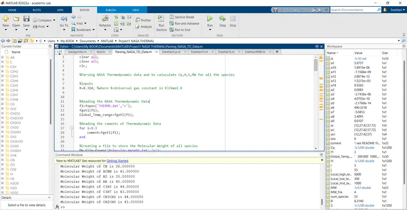
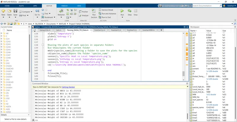
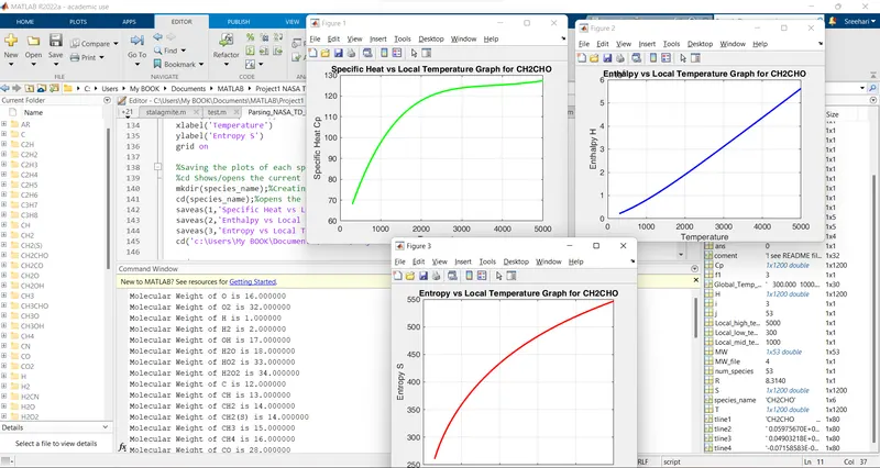
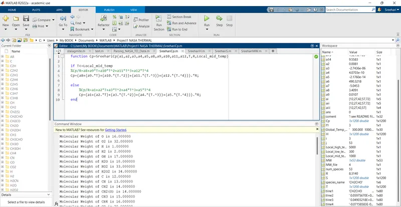
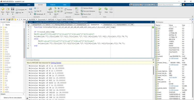
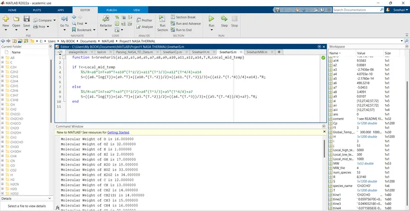
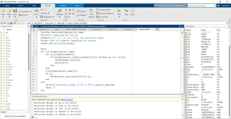
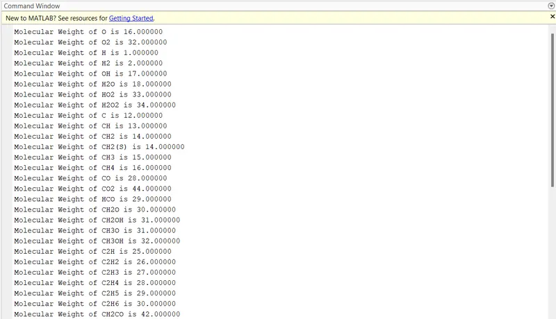
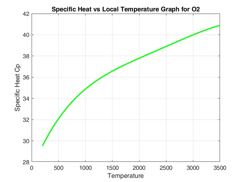
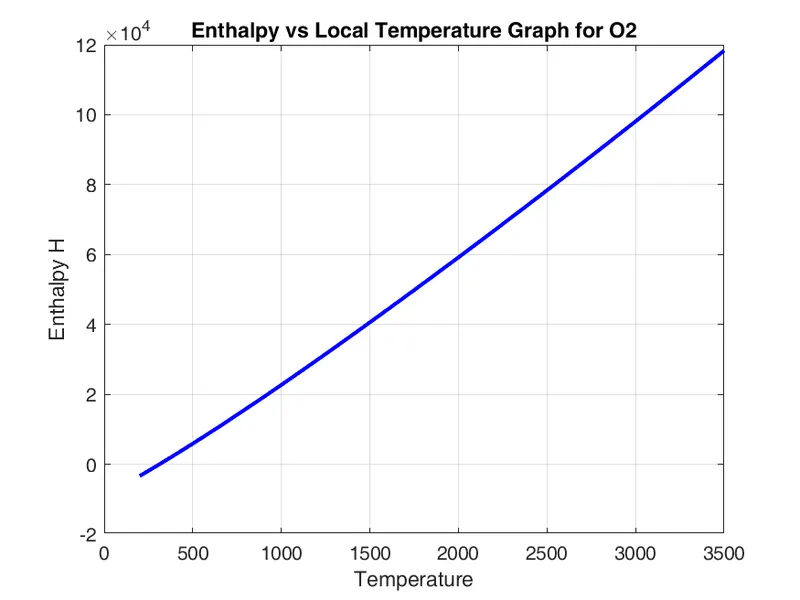
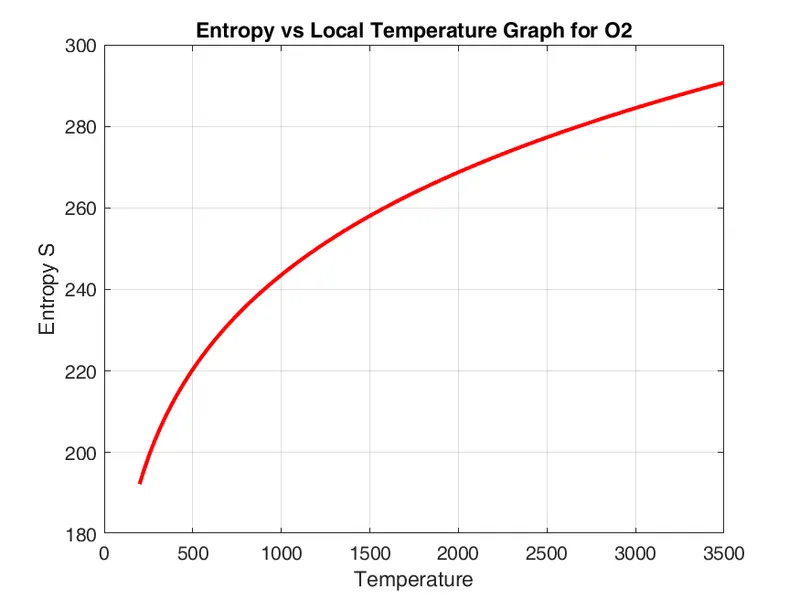
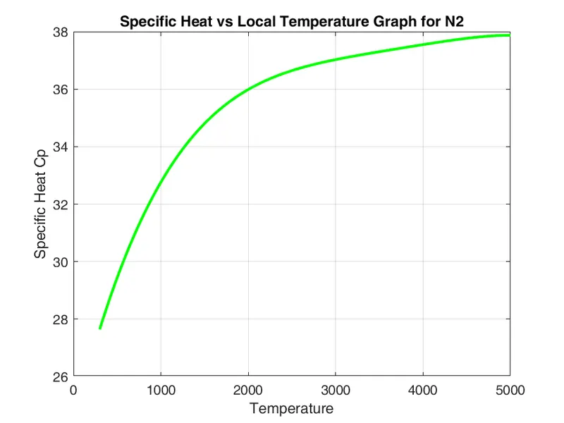
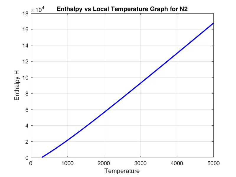
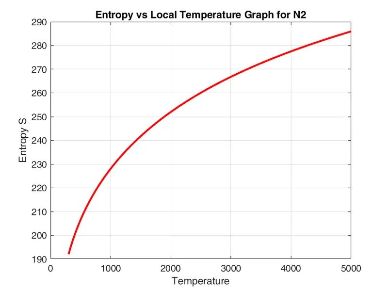
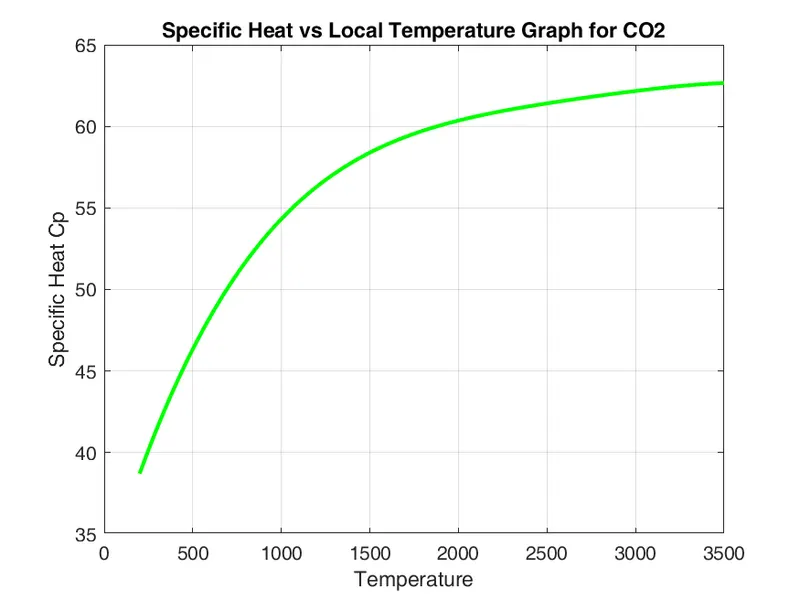
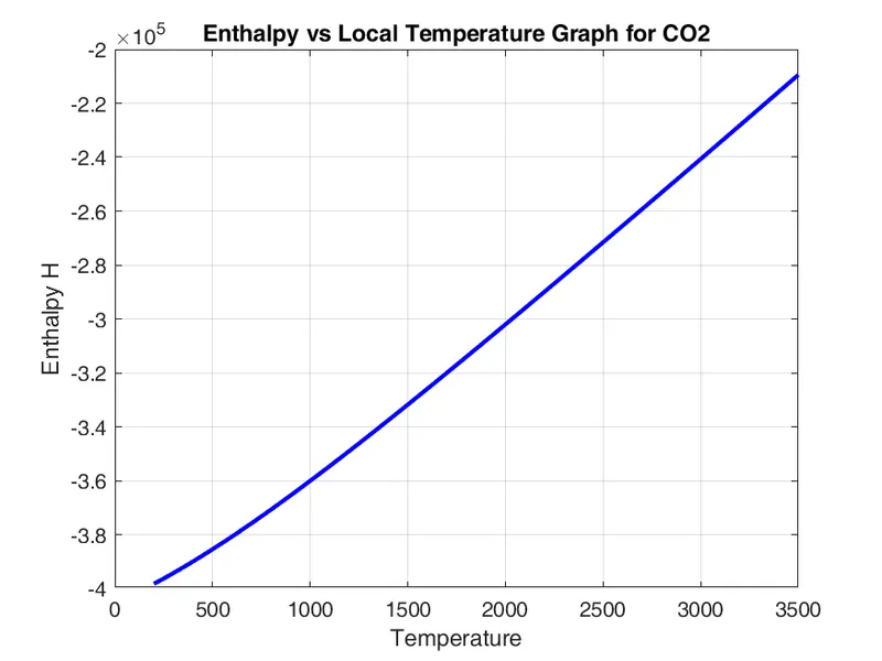
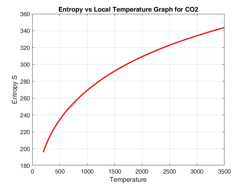
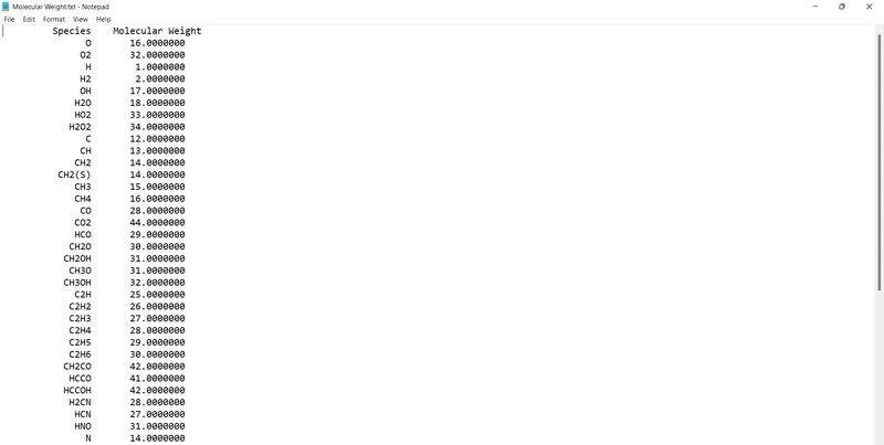
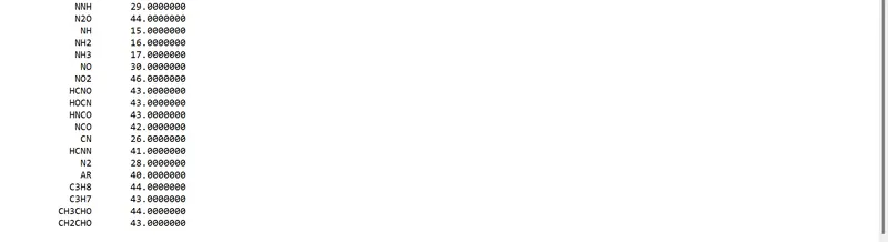
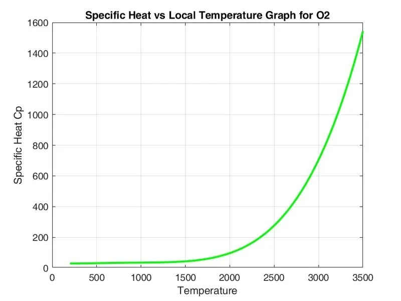
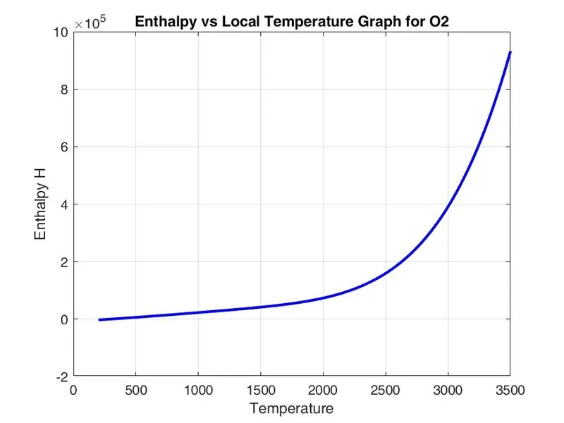
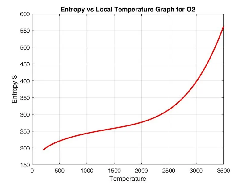
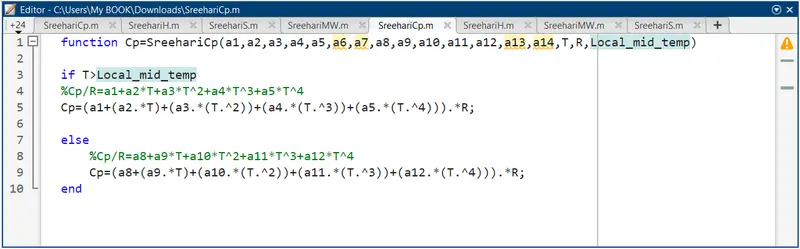
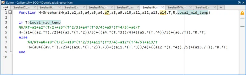
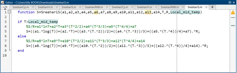
As can be inferred from the images shown above, I used the if condition as 'if T>Local_mid_temp' rather than 'if T<=Local_mid_temp'

So as I run my main code the if statement was being false continuously for almost half of the initial values of T(Low Local Temperature:High Local Temperature) till T=Local_mid_temp.Since half of the initial values are not satisfying the if statement, the function code tries to push values which satisfy the if statement forward and tries to take them as the initial values of the function.Because of this, the arrays of Cp,H,S will be wrong, as a result of which we get wrong plots.This might not happen if the arrays are small or when the polynomial equations are not much complex.

9.Methods to overcome the error: This error was solved easily by changing the if statement as if 'T<=Local_mid_temp' and rewriting the function codes as shown in the sections 5.2 to 5.4 of this report.

10.Results:

1. Wrote a code in Matlab to parse the NASA thermodynamic data file and used it to evaluate the thermodynamic properties(Cp,H,S) of the given gas species.
2. Calculated the molecular weight of each species and displayed it in the command window.
3. Created a file 'Molecular Weight.txt' to save the molecular weight of all the species.
4. Made plots of Cp,Enthalpy,Entropy vs Local Temperature Range specific for each species.
5. Included commands in the main program code to automatically save the plots as images with appropriate names and store them in separate folders for each species with the respective species name.
6. Google drive link for the folder containing plots for each species:
   https://drive.google.com/drive/folders/17l6Cfzk541LCGKnrdtOJUuOt_qQIsvND?usp=sharing
   

11.Conclusions: This program helped me to understand 'File Parsing' and how certain commands like cd,mkdir and saveas along with for loop can be used to automatically create and save information into different folders using Matlab.

12.References:

1. https://www.mathworks.com/help/matlab/ref/mkdir.html
2. https://www.mathworks.com/help/matlab/ref/strcmp.html
3. https://in.mathworks.com/help/matlab/ref/cd.html