Week 3 - Solving second order ODEs

Program:Solving Second Order ODE using Matlab and to Simulate a Simple Pendulum Motion

1.Aim: To solve a second order ODE and to simulate a Simple Pendulum Motion using Matlab.

2.Theory:

2.1 Differential Equations:

Differential equations arise from many problems in oscillations of mechanical and electrical systems, bending of beams,conduction of heat etc. Differential equations are used to model physical systems. The systems which change with time are called Dynamic systems. Examples are the models which describe heat transfer,electronic circuits with time dependent current and voltages. A differential equation involves differential coefficients or differentials.

An Ordinary Differential Equation(ODE) is one in which all the differential coefficients have reference to a single independent variable. In contrary, a Partial Differential Equation is one in which there will be two or more independent variables and partial differential coefficients with respect to any of them.The order  of a differential equation is the order of the highest derivative appearing in it.The degree of a differential equation is the degree of highest derivative occuring in it, when the equation has been expressed in a form free from radicals and fractional powers as far as derivatives are concerned.

2.2 Simple Pendulum:

In engineering, ODE is used to describe transient behaviour of a system such as simple pendulum.Unlike a compound pendulum, a simple pendulum has a bob shaped mass(m), connected to a string/rod of length L which is pivoted at the other end. When the bob is disturbed from it's initial equilibrium position by application of a force/couple which is removed after providing the initial displacement, the pendulum starts to oscillate on its own and eventually comes to rest after some time. Hence, a simple pendulum falls under the category of Damped Free Vibrations. On the other hand, a compound pendulum is one which can have any arbitrary shaped mass instead of a bob.

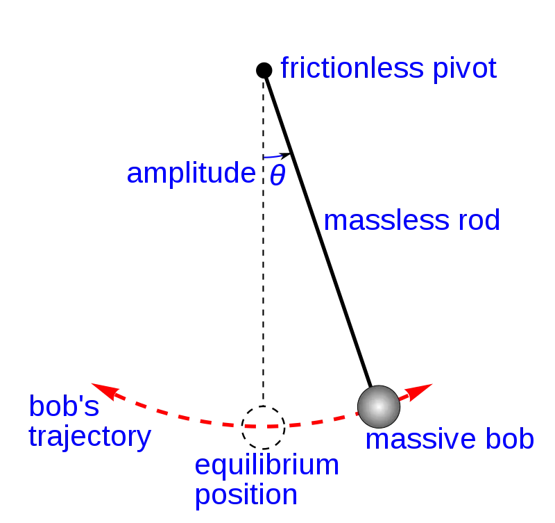
3.Governing Equations:

3.1Equation of motion of simple pendulum:

Any Damped Mechanical Vibration will have the following system parameters:

1. Inertia(`mddotx`) which is the resistance to change of state and it deals with Kinetic energy.
2. Damping(`bdotx`) which is the property of the system due to which it resists relative motion and this leads to loss of energy.
3. Restoration(`kx`) which is the property by which the body always returns to it's initial equilibrium position.It deals with Potential energy.

                where m represents mass(kg), b represents damping coefficient(Ns/m) and k is the spring constant(N/m).

The step by step procedure to derive the equation of motion for a simple pendulum using Newton's Method/D'Alembertz Principle is described below:

1. Recognize the system:

         System- Simple pendulum

     b.Decide the displacement variable(either x or `theta` or both):

         Displacement variable=`theta` (since, angular displacement takesplace)

     c.Identify the Equilibrium position

     d.Provide a small displacement to the mass from it's initial equilibrium position and draw the Free Body Diagram(FBD) at  the displaced          position.

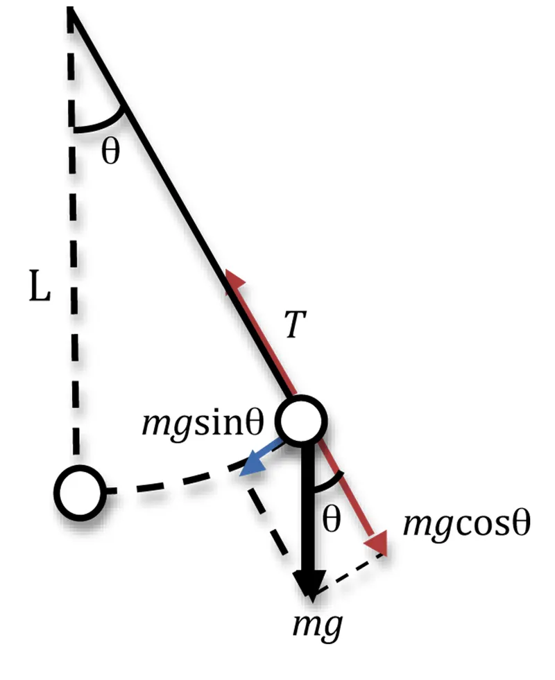
     e.Write Equation of Motion by Newton's Law/D'Alembertz Law:

         That is, `SigmaF_("external") =F_("inertia")`

               `implies SigmaF_("external")-(-F_("inertia"))=0`

               `implies SigmaF_("external")+F_("inertia")=0`................(i)

Solving equation (i), we get the Equation of Motion for a Simple Pendulum which is:

                `(d^2theta)/dt^2+b/m.(d theta)/dt+g/L.sin(theta)=0`..............(ii)

Now this is a Second Order ODE in '`theta`'

3.2Converting Second Order ODE into First Order ODE:

Equation (ii) is a Second Order ODE, but a Matlab program can include only First Order ODE. Therefore, we have to convert this equation into a First Order ODE as follows:

Let     `theta=theta_1`

      `(d theta)/dt=(d theta_1)/dt= theta_2`

    `(d^2 theta)/dt^2=(d^2 theta_1)/dt^2= (d theta_2)/dt`

Therefore equation (ii) becomes,

           `(d theta_2)/dt+b/m.theta_2+g/L.sin(theta_1)=0`

i.e,   `(d theta_1)/dt= theta_2`

        `(d theta_2)/dt= -b/m*theta_2-g/L*sin(theta_1)`

        `d/dt[theta_1 ; theta_2]`=[`theta_2 ; -b/m.theta_2-g/L.sin(theta_1)`

and let  `theta=[theta_1 ; theta_2]`

where `theta_1=`Angular Displacement of pendulum bob

            `theta_2=`Angular Velocity of pendulum bob

By solving the above equation in Matlab, we get angular displacement and angular velocity with respect to time.

4.Objectives:

1. To solve the equation of motion of simple pendulum with damping using Matlab.
2. To create an animation of simulation of this simple pendulum using Matlab.

5.Code:

5.1Main code:

clear all;
close all;
clc;

%Solving second order ODE using Matlab and to simulate a simple pendulum motion

%inputs: damping coefficient(b in Ns/m),length of pendulum(l in metres),acceleration due to gravity(g in m/s^2), mass(m in kg)
b=0.05;
l=1;
g=9.81;
m=1;

%initial conditions
theta_0=[0;3];

%time points
time_span=linspace(0,20,500);

%Solving ODE
[t,results]= ode45(@(t,theta)ode_func(t,theta,b,l,g,m),time_span,theta_0);

%plotting 2nd order ODE
figure(1)
hold on
plot(t,results(:,1))
plot(t,results(:,2))
xlabel('Time (s)')
ylabel('Angular displacement(rad) /Angular velocity (rad/s)')
legend('Angular displacement','Angular velocity')
grid on



%simulating pendulum motion
ct=1;
for i=1:length(time_span);
    beta=results(i,1);
    
    %coordinates of pendulum
    x0=0;
    y0=0;
    x1=l*sin(beta);
    y1=-l*cos(beta);

    figure(2)
    plot([-0.5 0.5],[0 0],'linewidth',8,Color=[0 0.6 0])
    hold on
    title('Motion of Simple Pendulum with Damping','Fontsize',20)
    plot(x0,y0,'.','Color','r')
    plot([x0 x1],[y0 y1])
    plot(x1,y1,'Marker','o','MarkerSize',10,'MarkerFaceColor','b')
    hold off
    axis([-1.7 1.7 -1.7 1.7]) 
    pause(0.03)
    M(ct)=getframe(gcf)
    ct=ct+1;

end

movie(M)
videofile=VideoWriter('Simulating_Pendulum.avi','Uncompressed AVI')
open(videofile)
writeVideo(videofile,M)
close(videofile)

 Explanation of Main code: 

1. Firstly,I cleared the Workspace,Command window and closed all current plots using clear all,clc and close all commands. 
2. Inputs such as damping coefficient,length of pendulum,acceleration due to gravity and mass are defined. 
3. Initial angular displacement and angular velocity are defined using the command theta_0=[0;3] where 0 is the initial angular displacement and 3 represents the initial angular velocity.
4. 500 values of time are defined between 0-20 seconds using linspace() command. 
5. ode45 is an inbuilt Matlab function to solve non-stiff differential equations using medium order method.Therefore we call in the function ode_func(t,theta,b,l,g,m) ,which has been defined earlier, using the solver ode45 defined as [t,results]= ode45(@(t,theta)ode_func(t,theta,b,l,g,m),time_span,theta_0). This would integrate the differential equation y'=f(t,results) from t0 to tf with initial condition theta_0. Here ode45(@(t,theta) is used to show that the matrix [t,results] is defined at (t,theta).The solution will be stored in [t,results] which is a 500x3 matrix with 't' being a '500x1' and 'results' being '500x2' matrices. The first column of results represent angular displacements and second column represents angular velocities. 
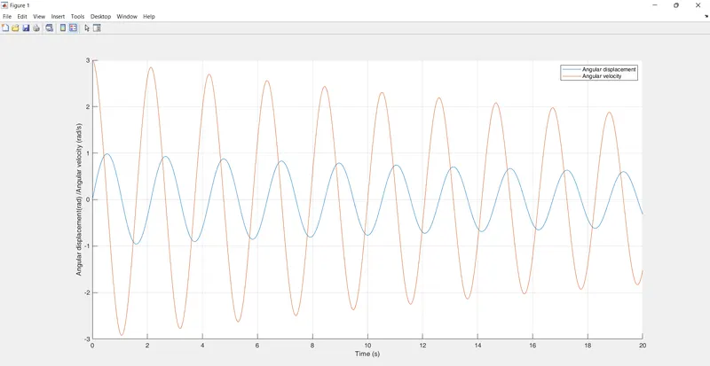
6. In next step, we plot angular diplacement and velocity with respect to time.For this we use hold on command so that all the plot() commands are executed. Firstly, we plot time vs angular displacement(radian), so the plot() command is given as plot(t,results(:,1)) which means all the rows in first column of [results] is considered. To plot time vs angular velocity, we should use plot(t,results(:,2)) so that all rows of only the second column of [results] are considered.Then, xlabel() and ylabel() commands are used to label x and y axes respectively and legend() command is used to label the curves.Finally grid on is used.
7. The next procedure is to create an animation of simulation of simple pendulum.For this Iam defining the first frame as ct=1 followed by a for loop. Inside the for loop I have defined 
   i=1:length(time_span);

   beta=results(i,1);

    

   Then x and y coordinates of pendulum are defined as  

    

   x0=0;

   y0=0;

   x1=l*sin(beta);

   y1=-l*cos(beta);

    

   Now the plot of simple pendulum is to be made as follows:

    

   figure(2)

   plot([-0.5 0.5],[0 0],'linewidth',8,Color=[0 0.6 0])

   hold on

   title('Motion of Simple Pendulum with Damping','Fontsize',20)

   plot(x0,y0,'.','Color','r')

   plot([x0 x1],[y0 y1])

   plot(x1,y1,'Marker','o','MarkerSize',10,'MarkerFaceColor','b')

   hold off

   axis([-1.7 1.7 -1.7 1.7])

   pause(0.03)

   M(ct)=getframe(gcf)

   ct=ct+1;

   end

    
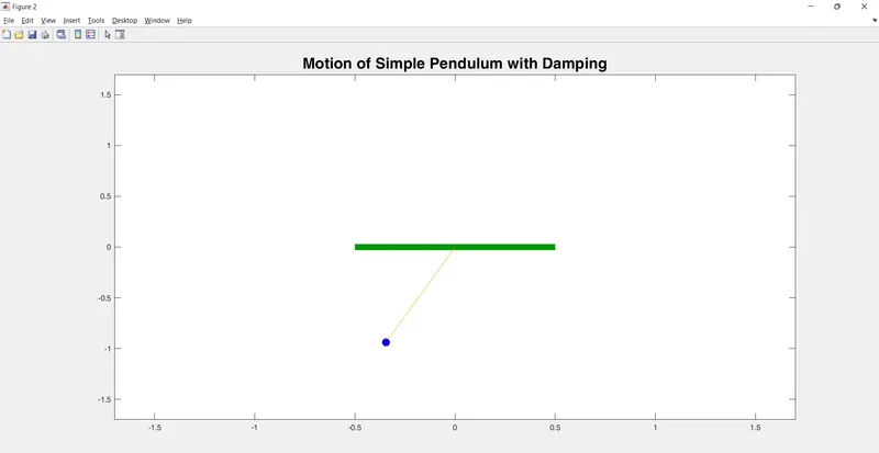
   Here, the first plot() command is used to create a line to replicate the wall on which the pendulum hangs. hold on command is used so that all the plot() commands appear in the graph. Title is given using title() command followed by plot() commands to mark the length and bob of pendulum. Here pendulum bob is created using 'Marker' command inside the plot() command.The size and color of bob are defined using 'MarkerSize' and 'MarkerFaceColor' commands respectively.This is followed by hold off, axis() and pause() commands.The frame so plotted is stored in an array M(ct) and ct value is incremented by 1 using ct=ct+1.for loop is terminated using end command.
8. All the frames so plotted are animated and stored as a video using the commands:

                        The videofile should be saved in '.avi' format as 'Uncompressed AVI'.                                                            

5.2 Function code:                                                                                                                                                       

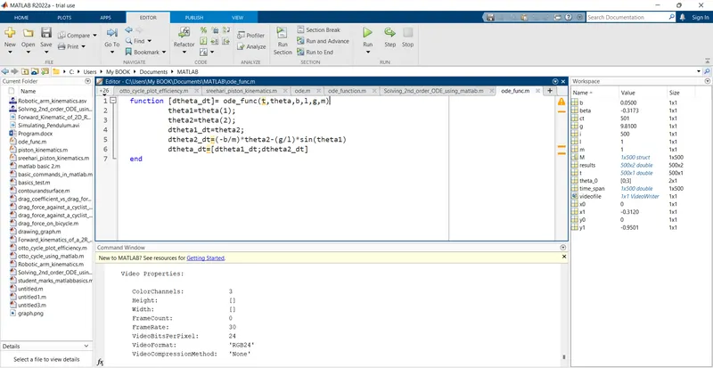
function [dtheta_dt]= ode_func(t,theta,b,l,g,m)
         theta1=theta(1);
         theta2=theta(2);
         dtheta1_dt=theta2;
         dtheta2_dt=(-b/m)*theta2-(g/l)*sin(theta1)
         dtheta_dt=[dtheta1_dt;dtheta2_dt]
end

 Explanation of Function code:

1. Here we are creating a function [dtheta_dt]= ode_func(t,theta,b,l,g,m) in order to convert the second order ODE into 2 first order ODEs to be solved by Matlab.Here theta is a column vector containing theta1 and theta2 where theta1 represents angular displacement in radians and theta2 is the angular velocity in radian/second.                            dtheta_dt is defined as 

       dtheta_dt=[dtheta1_dt;dtheta2_dt] where 

 

       dtheta1_dt=theta2;

       dtheta2_dt=(-b/m)*theta2-(g/l)*sin(theta1) and 

 

       theta1=theta(1);

       theta2=theta(2);

       Finally we end the function command.

 

       Now we call this fuction in the main code and solve it using the solver ode45().

 

 

6.Output Window:

6.1Main code:  

 

6.2 Function code:

 

7.Graphs:

7.1 Plot of Time vs Angular Displacement,Angular Velocity:

Here, the blue curve represents "Time vs Angular displacemet(rad)" and red curve represents "Time vs Angular velocity(rad/sec)".It can be observed that the amplitude of both Angular displacement and Angular velocity reduces with respect to time. It is due to loss of energy due to damping.

 

7.2 Simulation of Simple Pendulum:

The above figure shows one of the frames of the animation of simple pendulum.The angular motion of the pendulum would decrease with respect to time due to damping,which can be observed in the video given below:

 

 

8.Errors while programming:

 I encountered two errors while programming the code.Both these errors occured at once as shown below:

 

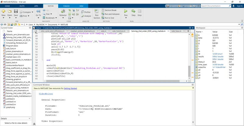
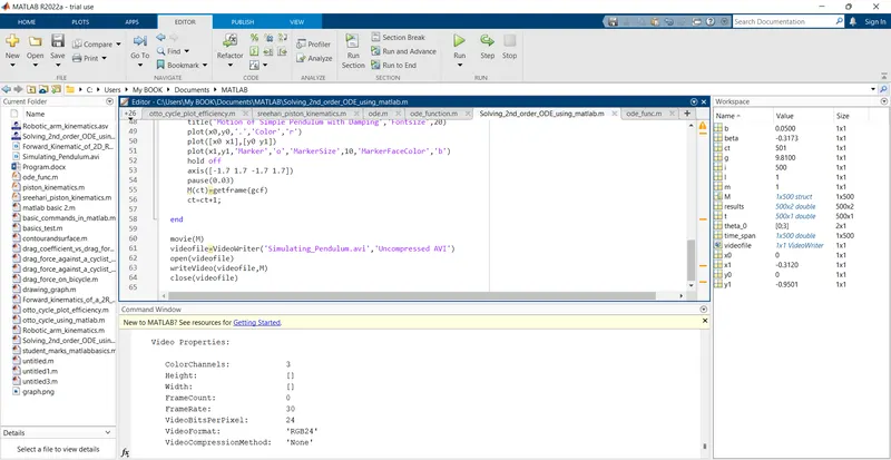
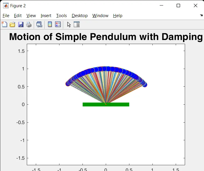
1. Since I hadn't used 'hold off' command following 'hold on' command all the frames were being plotted one after the other producing a plot as shown above. This was corrected by adding 'hold off' command in the main program.
2. Also I got an inverted plot by defining y1 coordinate as y1=l*cos(beta). This was solved by introducing a negative sign to y1 value as 'y1=-l*cos(beta)'.

9.Results:

1. Solved equation of motion for a damped simple pendulum and plotted the variation of angular displacement and velocity with respect to time.
2. Created an animation of a simple pendulum with damping coefficient b=0.05Ns/m.                                                        https://www.youtube.com/watch?v=CLu1B_paSCY    

10.Conclusions:

1. Understood that any higher order ODEs can be solved using Matlab by converting them to a number of first order ODEs.
2. Integration of first order ODEs can be performed using ode45 command.
3. Simulation of a simple pendulum can be carried out in Matlab by knowing the variations in it's position with respect to time.