Week 4.1 - Genetic Algorithm

Program:Global Maxima of Stalagmite Function using MATLAB

1.Aim: To use Genetic Algorithm and find Global Maxima of Stalagmite function using MATLAB.

2.Objectives:

1. To understand the concept of Genetic algorithm in Matlab.
2. To use Genetic Algorithm and optimise the Stalagmite function for Global maximum.

3.Theory: Genetic Algorithm(GA) is a stochastic global search method that mimics the metaphor of natural biological evolution. GAs operate on a population of potential solutions applying the principle of the "survival of the fittest" to produce better and better approximations to a solution. At each generation, a new set of approximations is created by the process of selecting individuals according to their level of fitness in the problem domain and breeding them together using operators borrowed from natural genetics.This leads to evolution of populations of individuals that are better suited to their environment than the individuals they were created from, just as in natural adaptation. Individuals or current approximations,are encoded as strings,chromosomes, composed over some alphabets, so that the genotypes(chromosome values) are uniquely mapped onto the decision variable(phenotypic) domain.

The following flowchart summarizes how the Genetic Algorithm works:

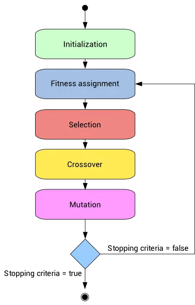
1. Initialization:
   The algorithm generally starts with randomly generated solutions. The size of the solutions depends on the nature of the problems. Individual solutions are generally represented by a “genotype” which is processed in software to produce an evaluable “Phenotype”. The genotype is the solution's manipulatable representation, while the phenotype is an evaluable solution to the problem.A genotype chromosome is represented by a software data structure such as a string of bits, characters, integers or real numbers.
   
   
2. Fitness assignment:
   Fitness function is the function which we have to optimise and its optimization is done with the help of number of generations which have been formed by the code in accordance with the fitness values of each member generated.These fitness values are used for reproduction of children.The GA scores each member of the current population by computing its fitness value known as the 'raw fitness scores'. These raw fitness scores are scaled into more usable range of values and form 'expectation values'. Later, the parents are selected based on these expectation values.
   
   
3. Selection:
   The idea of selection phase is to select the fittest individuals as 'parents' and let them pass their genes to the next generation. The main goal of this phase is to find the region where the chances of getting the best solution are more. Inspiration for this is from the survival of the fittest. It should be a balance between exploration and exploitation of search space. GA tries to move the genotype to higher fitness in the search space. Too strong fitness selection can lead to sub-optimal solutions,while too little fitness selection can bias the results towards unfocussed search.
   
   
4. Reproduction:
   The parents selected by the GA reproduces majorly in two ways:
   
   1)Crossover: Crossover is the most significant stage in GA. During crossover, a random point is selected while mating a pair of parents to generate offspring. There are 3 major types of crossover.
   
   a)Single Point Crossover: A point on both parents’ chromosomes is picked randomly, and designated as ‘crossover point’.
   b)Two-Point Crossover: Two crossover points are picked randomly from the parent chromosomes.
   c)Uniform Crossover: In a uniform crossover, typically, each bit is chosen from either parent with equal probability.
   
   eg: Parent1= 1 0 0 1 0 1 1 0
   Parent2= 1 0 1 1 1 0 0 0
   Here if single point crossover takesplace at an integer position i=5, the offsprings generated will be:
   Offspring1= 1 0 0 1 0 0 0 0 and
   Offspring2= 1 0 1 1 1 1 1 0
   
   2)Mutation: In a few new offsprings formed, some of their genes can be subjected to a mutation with a low random probability. This indicates that some of the bits in the bit chromosome can be flipped. Mutation happens to take care of diversity among the population and stop premature convergence.
   
   eg: Mutating the fourth bit of Offspring1 leads to the new string
   Offspring1(m)= 1 0 0 0 0 0 0 0
   
   Hence, genetic algorithm creates three types of children for the next generation namely elite, crossover and mutation children.Elites are the individuals in the current generation with the best fitness values. These individuals automatically survive to the next generation,Crossover are created by combining the vectors of a pair of parents and Mutation children are created by introducing random changes, or mutations, to a single parent.
   
   
5. Stopping criteria:
   

   The genetic algorithm uses the following options to determine when to stop.

   • MaxGenerations— The algorithm stops when the number of generations reaches MaxGenerations.
     
     
   • MaxTime— The algorithm stops after running for an amount of time in seconds equal to MaxTime.
     
     
   • FitnessLimit— The algorithm stops when the value of the fitness function for the best point in the current population is less than or equal to FitnessLimit.
     
     
   • MaxStallGenerations— The algorithm stops when the average relative change in the fitness function value over MaxStallGenerations is less than Function tolerance.
     
     
   • MaxStallTime— The algorithm stops if there is no improvement in the objective function during an interval of time in seconds equal to MaxStallTime.
     
     
   • FunctionTolerance— The algorithm runs until the average relative change in the fitness function value over MaxStallGenerations is less than Function tolerance.
     
     
   • ConstraintTolerance— The ConstraintTolerance is not used as stopping criterion. It is used to determine the feasibility with respect to nonlinear constraints. Also, max(sqrt(eps),ConstraintTolerance) determines feasibility with respect to linear constraints.

   The algorithm stops as soon as any one of these conditions is met and the solution obtained is the optimal solution. If none of these conditions are met, GA goes back to Fitness Assignment.

Syntax for Genetic Algorithm is described below:

x = ga(fun,nvars)
x = ga(fun,nvars,A,b)
x = ga(fun,nvars,A,b,Aeq,beq)
x = ga(fun,nvars,A,b,Aeq,beq,lb,ub)
x = ga(fun,nvars,A,b,Aeq,beq,lb,ub,nonlcon)
x = ga(fun,nvars,A,b,Aeq,beq,lb,ub,nonlcon,options)
x = ga(fun,nvars,A,b,Aeq,beq,lb,ub,nonlcon,intcon)
x = ga(fun,nvars,A,b,Aeq,beq,lb,ub,nonlcon,intcon,options)
x = ga(problem)
[x,fval] = ga(___)
[x,fval,exitflag,output] = ga(___)
[x,fval,exitflag,output,population,scores] = ga(___)

• x = ga(fun,nvars) finds a local unconstrained minimum, x, to the objective function, fun. nvars is the dimension (number of design variables) of fun.

• x = ga(fun,nvars,A,b) finds a local minimum x to fun, subject to the linear inequalities A*x ≤ b. ga evaluates the matrix product A*x as if x is transposed (A*x').
  
  
• x = ga(fun,nvars,A,b,Aeq,beq) finds a local minimum x to fun, subject to the linear equalities Aeq*x = beq and A*x ≤ b. (Set A[] and b[] if no linear inequalities exist.) ga evaluates the matrix product Aeq*x as if x is transposed (Aeq*x').
  
  
• x = ga(fun,nvars,A,b,Aeq,beq,lb,ub) defines a set of lower and upper bounds on the design variables, x, so that a solution is found in the range lb ≤ x ≤ ub. (Set Aeq=[] and beq=[] if no linear equalities exist.)
  
  
• x = ga(fun,nvars,A,b,Aeq,beq,lb,ub,nonlcon) subjects the minimization to the constraints defined in nonlcon. The function nonlcon accepts x and returns vectors C and Ceq, representing the nonlinear inequalities and equalities respectively. ga minimizes the fun such that C(x) ≤ 0 and Ceq(x) = 0. (Set lb=[] and ub=[] if no bounds exist.)
  
  
• x = ga(fun,nvars,A,b,Aeq,beq,lb,ub,nonlcon,options) minimizes with the default optimization parameters replaced by values in options. (Set nonlcon=[] if no nonlinear constraints exist.) Create options using optimoptions.
  
  
• x = ga(fun,nvars,A,b,Aeq,beq,lb,ub,nonlcon,intcon) or x = ga(fun,nvars,A,b,Aeq,beq,lb,ub,nonlcon,intcon,options) requires that the variables listed in intcon take integer values.
  
  
• x = ga(problem) finds the minimum for problem, a structure described in problem.
  
  
• [x,fval] = ga(___), for any previous input arguments, also returns fval, the value of the fitness function at x. We have used this syntax in our code.
  
  
• [x,fval,exitflag,output] = ga(___) also returns exitflag, an integer identifying the reason the algorithm terminated, and output, a structure that contains output from each generation and other information about the performance of the algorithm.
  
  
• [x,fval,exitflag,output,population,scores] = ga(___) also returns a matrix population, whose rows are the final population, and a vector scores, the scores of the final population.
  
  

GA finds it's application in many engineering applications like solving global optimization problems, optimal design of aerodynamic bodies in complex flowfields etc.

4.Governing Equations:

4.1 Stalagmite Function:

`f(x,y)=f_(1,x).f_(2,x).f_(1,y).f_(2,y)`

`f_(1,x)=[sin(5.1pix+0.5)]^6`

`f_(1,y)=[sin(5.1piy+0.5)]^6`

`f_(2,x)=exp[-4ln(2)(x-0.0667)^2/0.64]`

`f_(2,y)=exp[-4ln(2)(y-0.0667)^2/0.64]`

• A stalagmite is an upward growing mound of mineral deposites that have precipitated from water dripping onto the floor of a cave. Most stalagmites have rounded or flattened tips.
• A stalagmite function generally refers to the function with which we are generating values over a stalagmite kind of surface for finding out the local and global maxima and minima of that particular given function.
• For this in Matlab we are using a method called 'Optimization'. It is a programming which does a selection of the best element with regard to some criterion from some set of population.
• Optimization is done by systematically choosing input values ​​from within an allowed set and computing the results of the function.
• In matlab to perform optimization we use 'Genetic Algorithm' method which is an inbuilt function in matlab to find the global maxima of that given stalagmite function.
  
  
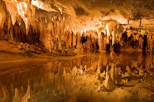
  Figure4.1 : Stalagmites

5.Code:

5.1 Main Code:

clear all;
close all;
clc;

%Defining Searchspace
x=linspace(0,0.6,150);
y=linspace(0,0.6,150);
num_cases=50;

%Creating a 2D Mesh
[xx yy]=meshgrid(x,y);

%Evaluating the Stalagmite Function
for i=1:length(xx);
    for j=1:length(yy);
        input_vector(1)=xx(i,j);
        input_vector(2)=yy(i,j);
        f(i,j)=stalagmite(input_vector);
    end
end

tic
%Study1- Statistical behaviour with unbounded inputs
for i=1:num_cases
[inputs,f_optimum(i)]=ga(@stalagmite,2);
x_optimum(i)=inputs(1);
y_optimum(i)=inputs(2);

end
Study1_time=toc

figure(1)
subplot(2,1,1)
surfc(xx,yy,-f)
shading interp
hold on
plot3(x_optimum,y_optimum,-f_optimum,'Marker','o','MarkerSize',5,'MarkerFaceColor','r')
title('Unbounded Inputs')
xlabel('x value')
ylabel('y value')
zlabel('Function -f')

subplot(2,1,2)
plot(-f_optimum)
xlabel('Iterations')
ylabel('Function Maximum')


tic
%Stydy 2- Statistical behaviour with upper and lower bounds
for i=1:num_cases
    [inputs,f_optimum(i)]=ga(@stalagmite,2,[],[],[],[],[0;0],[0.8;0.8]);
    x_optimum(i)=inputs(1);
    y_optimum(i)=inputs(2);
end
Study2_time=toc

figure(2)
subplot(2,1,1)
surfc(xx,yy,-f)
shading interp
hold on
plot3(x_optimum,y_optimum,-f_optimum,'Marker','o','MarkerSize',5,'MarkerFaceColor','r')
title('Bounded Inputs')
xlabel('x value')
ylabel('y value')
zlabel('Function -f')

subplot(2,1,2)
plot(-f_optimum)
xlabel('Iterations')
ylabel('Function Maximum')


tic
%Study 3- Increasing the size of GA Initial Population

options=optimoptions('ga','PopulationSize',500);
for i=1:num_cases
    [inputs,f_optimum(i)]=ga(@stalagmite,2,[],[],[],[],[0;0],[0.8;0.8],[],[],options);
    x_optimum(i)=inputs(1);
    y_optimum(i)=inputs(2);
end
Study3_time=toc

figure(3)
subplot(2,1,1)
surfc(xx,yy,-f)
shading interp
hold on
plot3(x_optimum,y_optimum,-f_optimum,'Marker','o','MarkerSize',5,'MarkerFaceColor','r')
title('Bounded Inputs with Increased Population Size')
xlabel('x value')
ylabel('y value')
zlabel('Function -f')

subplot(2,1,2)
plot(-f_optimum)
xlabel('Iterations')
ylabel('Function Maximum')

Expanation of Main Code:

1. Firstly, we clear the Workspace, Command window and close all the plots using clear all,clc and close all commands respectively.
2. Then we define the Searchspace as 150 values each of x and y ranging from 0 to 0.6 using the linspace() command.I have also defined an array num_cases=50 which denotes the total number of times the genetic algorithm is to be run.
3. Then I converted x and y into 2 Dimensional arrays xx and yy (each having a size 150x150) using [xx yy]=meshgrid(x,y).
4. Now we evaluate the Stalagmite function which has been defined earlier in stalagmite.m file. (Important thing to be noted is that both the main code and the function(stalagmite) code should be saved in the same path.)To do this, we use for loop as follows:
   
   for i=1:length(xx);

   for j=1:length(yy);

   input_vector(1)=xx(i,j);

   input_vector(2)=yy(i,j);

   f(i,j)=stalagmite(input_vector);

   end

   end
   Here values of i and j ranges from 1 to 150(length of xx, yy) and a for loop is used for j within the for loop for i so that for each value of i, there will be 150 values for j. f(i,j)=stalagmite(input_vector) is used to call the stalagmite function where input_vector is defined as input_vector=[xx(i,j) yy(i,j)].Hence by running this for loop, we get f as 150x150 array.
5. From now we are going to use three studies to finally arrive at our optimised result.
   
   tic
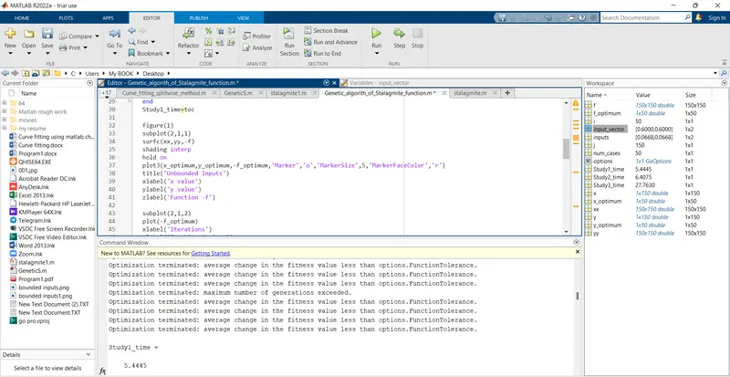
   %Study1- Statistical Behaviour

   for i=1:num_cases

   [inputs,f_optimum(i)]=ga(@stalagmite,2);

   x_optimum(i)=inputs(1);

   y_optimum(i)=inputs(2);

   end

   Study1_time=toc

   figure(1)

   subplot(2,1,1)

   surfc(xx,yy,-f)

   shading interp

   hold on

   plot3(x_optimum,y_optimum,-f_optimum,'Marker','o','MarkerSize',5,'MarkerFaceColor','r')

   title('Unbounded Inputs')

   xlabel('x value')

   ylabel('y value')

   zlabel('Function -f')

   subplot(2,1,2)

   plot(-f_optimum)

   xlabel('Iterations')

   ylabel('Function Maximum')
   
   In Study1, we are using ga to optimise the stalagmite function using "Unbounded Inputs". So firstly we use for loop to run the ga 50 times(num_cases). The syntax for Genetic Algorithm is given as [inputs,f_optimum(i)]=ga(@stalagmite,2). Here ga(@stalagmite denotes that the Genetic Algorithm is defined at the function named stalagmite and 2 represents the number of variables. Here inputs and f_optimum(i) represents the outputs, with the array [inputs] defined as [x_optimum(i) y_optimum(i)]. Since they are within the for loop, f_optimum, x_optimum and y_opyimum will be 1x50 arrays. Here tic-toc commands are used to denote the time taken to run the code. Now we plot figure(1) which is divided into 2x1 subplots. The command subplot(2,1,1) denotes that we are plotting the first subplot{i.e last number in the command subplot( , ,1)} in a plot which is having 2 rows and 1 column. So in the first subplot, we plot the Stalagmite function using surfc(xx,yy,-f). shading interp is used to avoid the grids/intersections on the surface plotted. Plot3() command is used to plot the points for x_optimum,y_optimum,-f_optimum for each case(iteration) and they are labelled/marked as 'o' using the 'Marker' command and the size , face color of marker are specified by 'MarkerSize' and 'MarkerFaceColor' commands respectively. The axes x,y,z are labelled using the commands xlabel(),ylabel() and zlabel() commands respectively. Here the title is given using title('Unbounded Inputs'). It's named 'Unbounded Inputs' because we haven't specified the bounds while defining the Genetic Algorith in the command [inputs,f_optimum(i)]=ga(@stalagmite,2). Next step is to make the second subplot using subplot(2,1,2) in which we plot -f_optimum. Here, it is very important to use plot(-f_optimum) and not plot(f_optimum) because by default ga always optimises the function for "global minima", since our area of interest is "global maxima" we should introduce -ve sign to f_optimum while making the plot. xlabel is given as Iterations and ylabel as Function Maximum. But from the output of study1(refer section7.1) we will come to know that f_optimum is spread all over in the range 0 to 1 during the 50 iterations and this is because we have not defined the upper and lower bounds for ga, as a result of which the populations ga take goes over the limits 0.6 and below 0 for the x and y values. Since f_optimum is not converging, Study1 is not giving optimised solution for global maxima. Hence we have to do Study2.
   
   
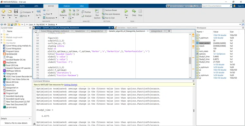
   tic

   %Stydy 2- Statistical behaviour with upper and lower bounds

   for i=1:num_cases

   [inputs,f_optimum(i)]=ga(@stalagmite,2,[],[],[],[],[0;0],[0.8;0.8]);

   x_optimum(i)=inputs(1);

   y_optimum(i)=inputs(2);

   end

   Study2_time=toc

   figure(2)

   subplot(2,1,1)

   surfc(xx,yy,-f)

   shading interp

   hold on

   plot3(x_optimum,y_optimum,-f_optimum,'Marker','o','MarkerSize',5,'MarkerFaceColor','r')

   title('Bounded Inputs')

   xlabel('x value')

   ylabel('y value')

   zlabel('Function -f')

   subplot(2,1,2)

   plot(-f_optimum)

   xlabel('Iterations')

   ylabel('Function Maximum')
   
   Study2 is almost identical to Study1 except that we are defining the upper and lower bounds for ga in Study2. This is done using the command [inputs,f_optimum(i)]=ga(@stalagmite,2,[],[],[],[],[0;0],[0.8;0.8]); We know that the general syntax for ga is [x ,fval]= ga(fun,nvars,A,b,Aeq,beq,lb,ub). Since we do not define any specific values for A,b,Aeq,beq we represnt them as [],[],[],[] in our code.Lower and Upper bounds lb and ub are given as [0;0] and [0.8;0.8] respectively.From the output of Study2(refer section 7.2), it can be observed that in most of the iterations, Function Maximum converges towards 1 but still there are some deviations.This can be solved by taking a larger size of initial population in ga as illustrated in Study3.
   
   
   tic

   %Study 3- Increasing the size of GA Initial Population

   options=optimoptions('ga','PopulationSize',500);

   for i=1:num_cases

   [inputs,f_optimum(i)]=ga(@stalagmite,2,[],[],[],[],[0;0],[0.8;0.8],[],[],options);

   x_optimum(i)=inputs(1);

   y_optimum(i)=inputs(2);

   end

   Study3_time=toc

   figure(3)

   subplot(2,1,1)

   surfc(xx,yy,-f)

   shading interp

   hold on

   plot3(x_optimum,y_optimum,-f_optimum,'Marker','o','MarkerSize',5,'MarkerFaceColor','r')

   title('Bounded Inputs with Increased Population Size')

   xlabel('x value')

   ylabel('y value')

   zlabel('Function -f')

   subplot(2,1,2)

   plot(-f_optimum)

   xlabel('Iterations')

   ylabel('Function Maximum')
   
   Here options=optimoptions('ga','PopulationSize',500); is used to increase the initial population size to 500. The command [inputs,f_optimum(i)]=ga(@stalagmite,2,[],[],[],[],[0;0],[0.8;0.8],[],[],options); is used to enter the defined options into ga. From the output of Study3(refer section 7.3), it is observed that the Global Maxima converges towards 0.99999985 approximately equals to 1 for all the iterations.
   

5.2 Function Code:

function f=stalagmite(input_vector)
x=input_vector(1);
y=input_vector(2);

f1_x=(sin(5.1*pi.*x+0.5)).^6;
f1_y=(sin(5.1*pi.*y+0.5)).^6;
f2_x=exp(-4*log(2).*((x-0.0667).^2./0.64));
f2_y=exp(-4*log(2).*((y-0.0667).^2./0.64));

f=-f1_x.*f2_x.*f1_y.*f2_y;

end

Expalantion of Function Code:

The Stalagmite function is defined as shown above using the function command and it is saved in the same path as main code.Here we have made use of the Governing equations of Stalagmite function but at the end, we have used

6.1 Main Code:

6.1.1 Study1:

6.1.2 Study 2:

6.1.3 Study 3:

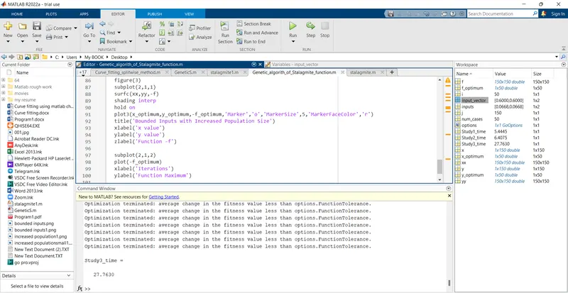
6.2 Function Code:

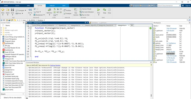
7.Graph:

7.1 Study1:

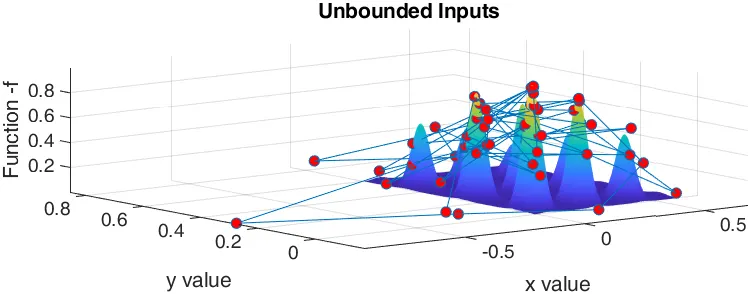
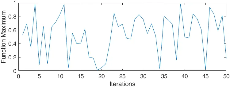
From the plots, it can be observed that the optimized value of function represented by 'Function Maximum' is varying between 0 and 1 over the 50 iterations. This is because we have not set lower and upper bounds for ga in the code as aresult of which the x and y values may go below 0 or above 0.6.

7.2 Study2:

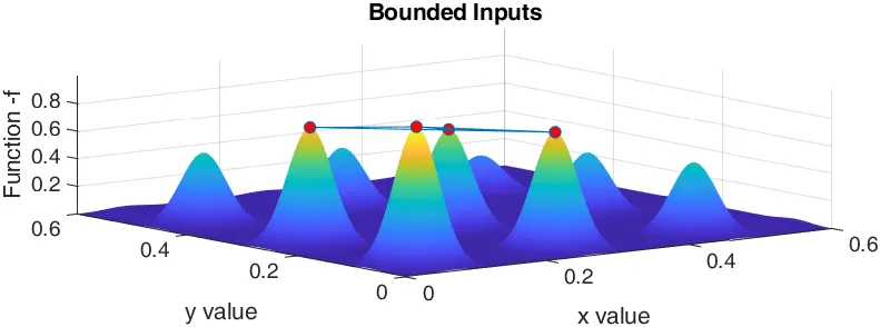
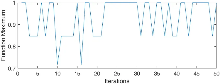
Now that we have defined the lower and upper bounds for ga as [0;0] and [0.8;0.8], we can see that the x and y values are restricted to the respective limits. We can also observe that the maximum value of the function is mostly equal to one, except for a few deviations over the entire iterations of ga. This can be solved by taking a larger size of initial population for ga.

7.3 Study3:

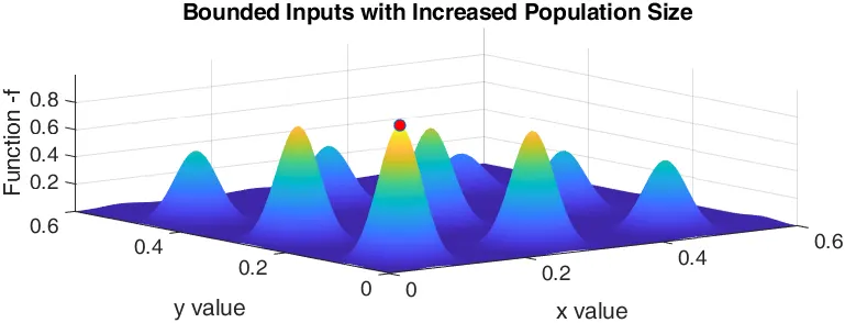
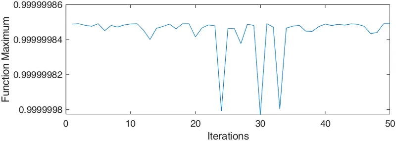
In Study 3 we have increased the initial population size of ga using the commands options=optimoptions('ga','PopulationSize',500); and [inputs,f_optimum(i)]=ga(@stalagmite,2,[],[],[],[],[0;0],[0.8;0.8],[],[],options); Hence the Global Maxima of the Stalagmite function converges to 0.99999985 which can be rounded off to 1.

8.Errors Faced while Programming:

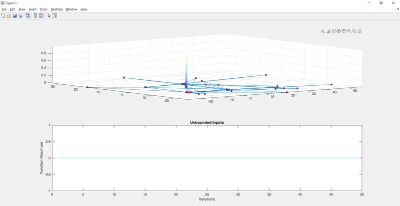
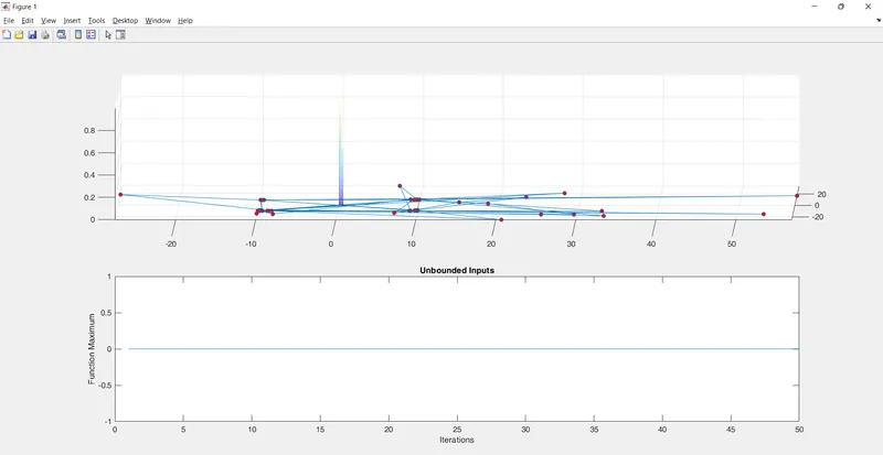
One major error which I faced is illustrated above. As is visible from the graph, I got an upward facing Stalagmite function but the problem was that all the -f_optimum values[Function Maximum values] evaluated by ga were equal to zero.

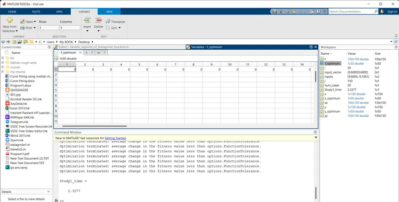
Why this happened is because I did not use negative sign in the equation of the stalagmite function f=-f1_x.*f2_x.*f1_y.*f2_y; and in surfc(xx,yy,-f); eventhough I put the negative sign in

plot3(x_optimum,y_optimum,-f_optimum,'Marker','o','MarkerSize',5,'MarkerFaceColor','r') and plot(-f_optimum)

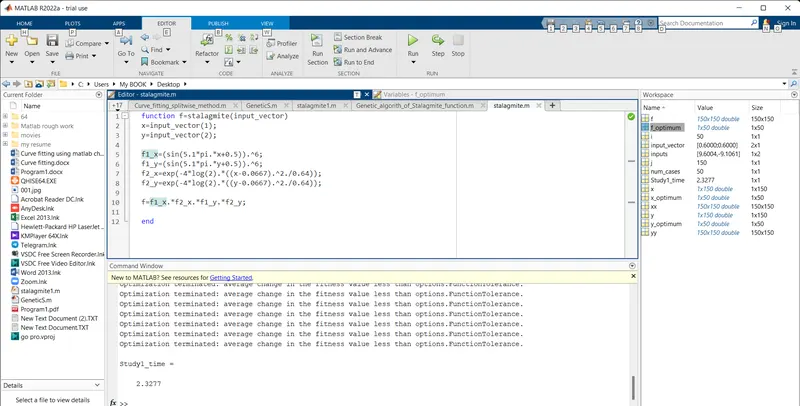
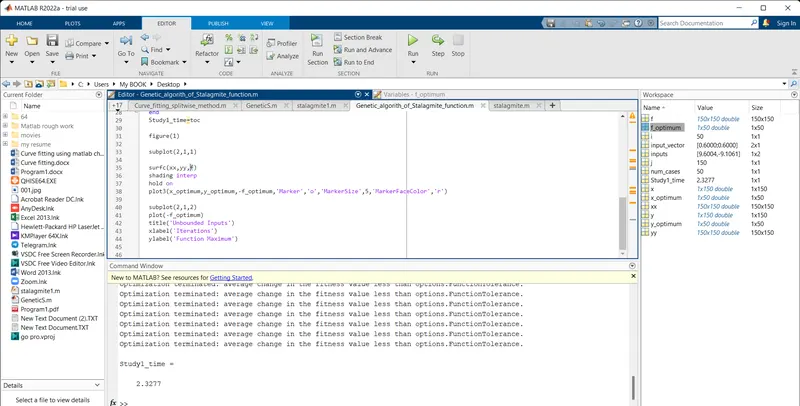
I thought that since we were plotting for an upward stalagmite function, there was no need for a negative sign in the equation f=f1_x.*f2_x.*f1_y.*f2_y; But what happened is that upon using surfc(xx,yy,f) for the defined f, the plot was coming out to be

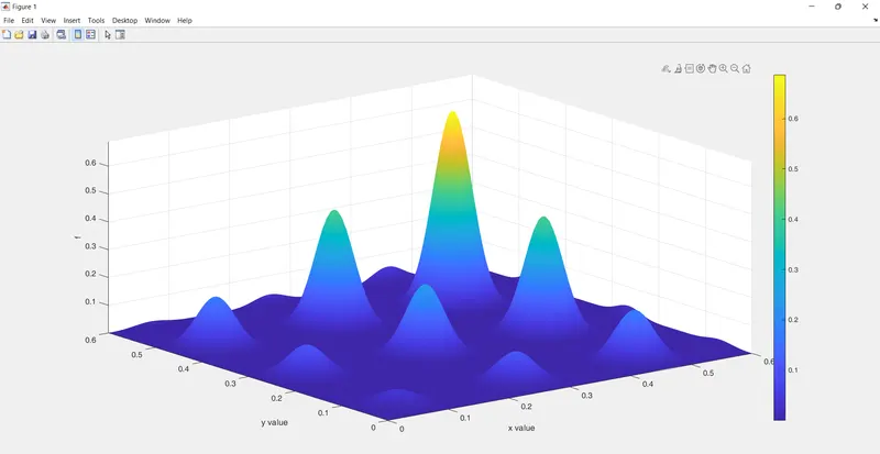
From here it is clearly visible that the minimum value of f is 0. We know that ga always optimizes for minimum value.So upon using the command [inputs,f_optimum(i)]=ga(@stalagmite,2), f_optimum takes up the minimum value,i.e, zero. Hence, even if we use

plot(-f_optimum), it would result in -0 which is 0 itself. This causes Function Maximum to tend towards zero throughout the iteration.

9.Methods to overcome the error:

The simple method adopted to overcome this error was to use -ve sign in the equation f=-f1_x.*f2_x.*f1_y.*f2_y so that it's maximum value becomes zero and minimum value becomes negative.Hence upon running the ga syntax, f_optimum now becomes a negative value. However, if we plot this using the surfc(xx,yy,f) command it would result in a downward stalagmite function. Thus to make the stalagmite function upward we have to use surfc(xx,yy,-f). Then for plotting the maximum value of f, we use plot(-f_optimum) so that -(-integer) turns out to be postive here rather than zero.

10.Results:

1. Used Genetic Algorith to optimize the Stalagmite function for Global Maxima, the value of which turned out to be `0.99999985 approx1``
2. The plot for 'Unbounded Inputs', 'Bounded Inputs' and 'Increased Population Size' were made.

11.Conclusions:

This challenge helped me to have a better understanding of Genetic Algorithm and how it can be used to obtain optimized results for stochastic problems based on the natural principle of 'Survival of the Fittest'.

12.References:

1. Genetic Algorithm TOOLBOX For Use with MATLAB by Andrew Chipperfield,Peter Fleming,Hartmut Pohlheim,Carlos Fonseca.
2. https://www.youtube.com/watch?v=96-u9s6D16k
3. https://in.mathworks.com/help/gads/how-the-genetic-algorithm-works.html
4. https://en.wikipedia.org/wiki/Genetic_algorithm#Initialization
5. https://towardsdatascience.com/introduction-to-genetic-algorithms-including-example-code-e396e98d8bf3