Week - 2 - Explicit and Implicit Analysis
Objective
Solve the following equation by using both implicit and explicit solution methods
`F(u)=u^3+9u^2+4u`
Theoretical Background
Explicit and Implicit methods are numerical approaches used to solve differential equations. Yet, they differ in the sense that explicit methods use the known information at the current time step to approximate the solution at the next time step, while implicit methods use both the information of the current and next time step, therefore, requiring to solve sets of more complex equations.
For instance, assuming an arbitrary function Y that varies with time (t):
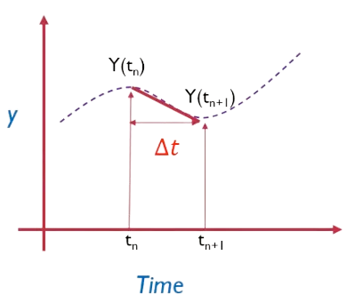
- Y value at time tn is known
- The slope Y' at time tn can be calculated
And we wish to know the value of Y at time n+1, the solution is given by the formula:
Both implicit and explicit methods start from this equation, yet, explicit methods assume that the slope y' is the one from the current time step, meanwhile, the implicit methods assume that the slope y' is the one from the next time step, resulting in the following equations:
Explicit:
`y_1=y_0+Δt∙y_0^′`
All values from the right hand side of the equation are known, thus, we can obtain y1 directly
Implicit
`y_1=y_0+Δt∙y_1^′`
Since y1 appears on both sides of the equations, we have to rely on other numerical methods such as Newton Raphson to solve this equation
In the context of FEA, we solve for the equation of motion, which is a second order partial differential equation:
`mu^(′′)+cu^′+ku=f(t)`
Where:
M: mass matrix
C: damping matrix
K: stiffness matrix
F: External force vector
U: Nodal displacement vector
U': Nodal velocity vector
U'': Nodal acceleration vector
The way of solving this equation is analogous to the previous case, yet, since we have a second order problem, we must solve a 2x2 system of equations
`u'_((n+1))=u_n^′+Δt∙u^(′′)`
`u_(n+1)=u_n+Δt∙u′`
If we use the velocities and accelerations from the known time step, we are solving by a explicit method. If we use the ones from the next time step with numerical methods, we are using a implicit method.
Procedure
Explicit Method
Starting by the explicit method, we can directly solve the problem by defining a force increment (1N) and deriving the equation with respect to u to obtain the slope. The problem then becomes:
`u_1=u_0+Δu`
Having the relation that `ΔF=K(u)∙Δu`
`Δu=(ΔF)/(K(u))`
`K(u)= (dF)/(du)=3u^2+18u+4`
`K(u_0 )=3(0)^2+18(0)+4=4`
`Δu=(ΔF)/(K(u)) =1/4`
`u_1=0+1/4=0.25`
`F(u_1 )=u_1^3+9u_1^2+4u_1=1.578`
Force Step 2
`u_2=u_1+Δu`
`K(u_1 )=3(0.25)^2+18(0.25)+4=8.6875`
`Δu=(ΔF)/(K(u_1 )) =1/8.6875=0.115`
`u_2=0.25+0.115=0.365`
`F(u_2 )=u_2^3+9u_2^2+4u_2=2.707`
Force Step 3
`u_3=u_2+Δu`
`K(u_2 )=3(0.365)^2+18(0.365)+4=10.967`
`Δu=(ΔF)/(K(u_2) ) =1/10.967=0.0911`
`u_3=0.365+0.0911=0.456`
`F(u_2 )=u_2^3+9u_2^2+4u_2=3.79`
To check the accuracy of our solution, we can compare the force step against the internal force, obtaining:
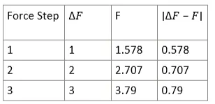
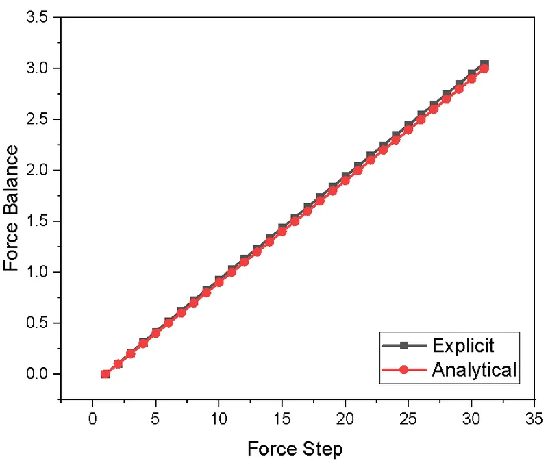
Therefore, we can see that one of the disadvantages of the explicit methods is that they induce inaccuracies that are dependent on the time step size. If we use a step size of 0.1, we get:
Implicit Method
The methodology to solve the problem by implicit methods starts the same as the previous case, yet, a residual parameter (R) is introduced along Newton-Raphson iterations to ensure the force step and the internal force are matching.
`u_1=u_0+Δu`
Having the relation that `ΔF=K(u)∙Δu`
`Δu=(ΔF)/(K(u))`
`K(u)= (dF)/(du)=3u^2+18u+4`
`K(u_0 )=3(0)^2+18(0)+4=4`
`Δu=(ΔF)/(K(u)) =1/4`
`u_1=0+1/4=0.25`
`F(u_1 )=u_1^3+9u_1^2+4u_1=1.578`
This R value is compared against a tolerance value (0.001), and in case that the value is larger than the tolerance, we have to use the following correction factor (derived from using Taylor Series)
`Δu_1=−K(u_1 )^(−1)∙R=−8.6875^(−1)∙0.578=−0.0665`
The updated value for the displacement and stiffness becomes
`u_1=u_1+Δu_1=0.25−0.0665=0.1835`
`k_(u1)=3(0.1835)^2+18(0.1835)+4=7.404`
From here, we have to recalculate the force values and repeat the criteria for the R value
`F(u_1 )=u_1^3+9u_1^2+4u_1=1.0433`
`R=abs(ΔF−F)=abs(1−1.0433)=0.0433>0.001`
Which means that we have to update our guess for the displacement once again
`Δu_1=−K(u_1 )^(−1)∙R=−7.404^(−1)∙0.0433=−0.00584`
`u_1=u_1+Δu_1=0.1835−0.00584=0.177`
By recalculating the force and R value we get:
`F(u_1 )=u_1^3+9u_1^2+4u_1=1.0003`
`R=abs(ΔF−F)=abs(1−1.0003)=0.0003<0.001`
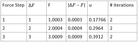
Since the residual condition is satisfied, we can proceed to calculate the displacement at the second and third force steps, resulting in:
Results
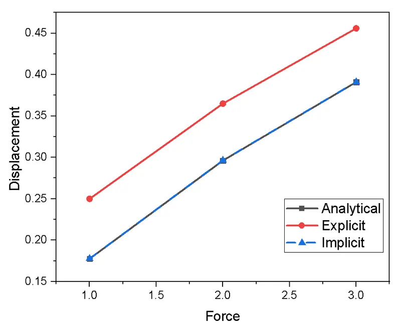
The final displacement vs force graph is plotted for both explicit and implicit methods against the analytical solution to the problem.
It can be observed that the implicit method provides an exact solution, while the explicit method overestimates the displacement in all cases. To overcome this, we could reduce the time step used for the solution at the expense of computational efficiency.
Therefore, implicit methods are recommended where large time steps can be used, such as quasi-static or dynamic problems that don't involve a large strain rate, in contrast, explicit methods are recommended in high strain events such as impact or drop tests.