Week 12 - Validation studies of Symmetry BC vs Wedge BC in OpenFOAM vs Analytical H.P equation

OBJECTIVE.

• To simulate an axis-symmetric laminar flow through the constant cross-sectional of the pipe by applying the symmetry boundary condition.
• To simulating for the mentioned angles i.e for 10, 25, 45 degrees using both symmetry and wedge boundary conditions and validate them with HP equations.

Theoretical Introduction:
Axi-symmetric flow: A flow pattern is axisymmetric when it is identical in every plane that passes through a certain straight-line. The straight-line in question is referred to as the symmetry axis.
Every longitudinal plane through the axis would exhibit the same streamline pattern.

Laminar Flow: In fluid dynamics, laminar flow is characterized by fluid particles following smooth paths in layers, with each layer moving smoothly past the adjacent layers with little or no mixing. At low velocities, the fluid tends to flow without lateral mixing, and adjacent layers slide past one another like playing cards. There are no cross-currents perpendicular to the direction of flow, nor eddies or swirls of fluids. In laminar flow, the fluid particles' motion is very orderly, with particles close to a solid surface moving in straight lines parallel to that surface.
Laminar flow is a flow regime characterized by high momentum diffusion and low momentum convection.
When a fluid flows through a closed channel such as a pipe or between two flat plates, either of two types of flow may occur depending on the fluid's velocity and viscosity: laminar flow or turbulent flow. Laminar flow occurs at lower velocities, below a threshold at which the flow becomes turbulent. The velocity is determined by a dimensionless parameter characterizing the flow called the Reynolds number, which also depends on the viscosity and density of the fluid and dimensions of the channel.

Procedure:

1. The procedure for this challenge involves editing the previously made MATLAB code and changing the input and the Boundary Conditions in OpenFoam. 


2. In the Automated BlockMeshDict file, we need to edit the wedge angle for one particular boundary condition. The angles at which we are performing the simulation and then later studying the simulation results are: 
a. 
10
o

b. 
25
o

c. 
45
o


The code for Wedge Boundary Condition at a wedge angle of 45 deg is as follows:
clear all
close all
clc

%Inputs:
l= 1.5;         %Length of the pipe.
theta = 45.0;    %Wedge angle.
d = 0.01;       %Diameter of the pipe.
c = 1.0;        %Conversion Factor. 
r = d/2;        %Radius of the Cylinder.
nx = 500;       %number of Mesh points in x-direction on the block.
ny= 25;         %Number of Mesh points in the y-direction on the block.
nz= 1;          %number of Mesh Points in the z-direction on the block.
gx = 1;         %Grading along the x-direction.
gy = 1;         %Grading along the y-direction.
gz = 1;         %Grading along the z-direction.


f1 = fopen('BlockMeshDict.txt','w');
fprintf(f1,'/*--------------------------------*- C++ -*----------------------------------*n');
fprintf(f1,'  =========                 | n');
fprintf(f1,'        /  F ield         | OpenFOAM: The Open Source CFD Toolbox n');
fprintf(f1,'       /   O peration     | Website:  https://openfoam.org n');
fprintf(f1,'      /    A nd           | Version:  8 n');
fprintf(f1,'     /     M anipulation  | n');
fprintf(f1,'/*------------------------------------------------------------------*/ n');
fprintf(f1, 'FoamFile n');
fprintf(f1,'{ n');
fprintf(f1,'    version     2.0; n');
fprintf(f1,'    format      ascii; n' );
fprintf(f1,'    class       dictionary; n');
fprintf(f1,'    object      blockMeshDict; n');
fprintf(f1,'} n');
fprintf(f1,'// * * * * * * * * * * * * * * * * * * * * * * * * * * * * * * * * * * * * * // n');

fprintf(f1,'convertToMeters %0.1f; n',c);
fprintf(f1,'n');
fprintf(f1,'vertices n');
fprintf(f1,'( n');
fprintf(f1,'(0 0 0) n');
fprintf(f1,'(%0.6f %0.6f %0.3f)n',r*sind(theta/2),r*cosd(theta/2),0);
fprintf(f1, '(%0.6f %0.6f %0.3f)n',-r*sind(theta/2),r*cosd(theta/2),0);
fprintf(f1,'(0 0 %0.3f) n',-l);
fprintf(f1,'(%0.6f %0.6f %0.3f)n',r*sind(theta/2),r*cosd(theta/2),-l);
fprintf(f1, '(%0.6f %0.6f %0.3f)n',-r*sind(theta/2),r*cosd(theta/2),-l);
fprintf(f1,'); n');
fprintf(f1,'n');

fprintf(f1,'blocks n');
fprintf(f1,'( n');
fprintf(f1,'hex (0 3 5 2 0 3 4 1) (%0.0f %0.0f %0.0f) simpleGrading (%0.0f %0.0f %0.0f) n',nx,ny,nz,gx,gy,gz);
fprintf(f1,'); n');
fprintf(f1,'n');

fprintf(f1,'edges n');
fprintf(f1,'( n');
fprintf(f1,'); n');
fprintf(f1,'n');

fprintf(f1,'boundary n');
fprintf(f1,'( n');
fprintf(f1,'in n');
fprintf(f1,'{ n');
fprintf(f1,'type patch; n');
fprintf(f1,'faces n');
fprintf(f1,'( n');
fprintf(f1,'(0 1 2 0) n');
fprintf(f1,'); n');
fprintf(f1,'} n');

fprintf(f1,'out n');
fprintf(f1,'{ n');
fprintf(f1,'type patch; n');
fprintf(f1,'faces n');
fprintf(f1,'( n');
fprintf(f1,'(3 5 4 3) n');
fprintf(f1,'); n');
fprintf(f1,'} n');

fprintf(f1,'ft n');
fprintf(f1,'{ n');
fprintf(f1,'type wedge; n');
fprintf(f1,'faces n');
fprintf(f1,'( n');
fprintf(f1,'(0 3 4 1) n');
fprintf(f1,'); n');
fprintf(f1,'} n');

fprintf(f1,'bk n');
fprintf(f1,'{ n');
fprintf(f1,'type wedge; n');
fprintf(f1,'faces n');
fprintf(f1,'( n');
fprintf(f1,'(3 0 2 5) n');
fprintf(f1,'); n');
fprintf(f1,'} n');

fprintf(f1,'top n');
fprintf(f1,'{ n');
fprintf(f1,'type wall; n');
fprintf(f1,'faces n');
fprintf(f1,'( n');
fprintf(f1,'(5 2 1 4) n');
fprintf(f1,'); n');
fprintf(f1,'} n');

fprintf(f1,'axis n');
fprintf(f1,'{ n');
fprintf(f1,'type empty; n');
fprintf(f1,'faces n');
fprintf(f1,'( n');
fprintf(f1,'(0 3 3 0) n');
fprintf(f1,'); n');
fprintf(f1, '} n');

fprintf(f1,'); n');
fprintf(f1,'n');

fprintf(f1,'mergePatchPairs n');
fprintf(f1,'( n');
fprintf(f1,'); n');
fprintf(f1,'n');
fprintf(f1,'// ************************************************************************* // n');


%END 


The code for Symmetry Boundary Condition at a wedge angle of 45 deg is as follows:
clear all
close all
clc

%Inputs:
l= 1.5;         %Length of the pipe.
theta = 45.0;    %Wedge angle.
d = 0.01;       %Diameter of the pipe.
c = 1.0;        %Conversion Factor. 
r = d/2;        %Radius of the Cylinder.
nx = 500;       %number of Mesh points in x-direction on the block.
ny= 25;         %Number of Mesh points in the y-direction on the block.
nz= 3;          %number of Mesh Points in the z-direction on the block.
gx = 1;         %Grading along the x-direction.
gy = 1;         %Grading along the y-direction.
gz = 1;         %Grading along the z-direction.


f1 = fopen('BlockMeshDict.txt','w');
fprintf(f1,'/*--------------------------------*- C++ -*----------------------------------*n');
fprintf(f1,'  =========                 | n');
fprintf(f1,'        /  F ield         | OpenFOAM: The Open Source CFD Toolbox n');
fprintf(f1,'       /   O peration     | Website:  https://openfoam.org n');
fprintf(f1,'      /    A nd           | Version:  8 n');
fprintf(f1,'     /     M anipulation  | n');
fprintf(f1,'/*------------------------------------------------------------------*/ n');
fprintf(f1, 'FoamFile n');
fprintf(f1,'{ n');
fprintf(f1,'    version     2.0; n');
fprintf(f1,'    format      ascii; n' );
fprintf(f1,'    class       dictionary; n');
fprintf(f1,'    object      blockMeshDict; n');
fprintf(f1,'} n');
fprintf(f1,'// * * * * * * * * * * * * * * * * * * * * * * * * * * * * * * * * * * * * * // n');

fprintf(f1,'convertToMeters %0.1f; n',c);
fprintf(f1,'n');
fprintf(f1,'vertices n');
fprintf(f1,'( n');
fprintf(f1,'(0 0 0) n');
fprintf(f1,'(%0.6f %0.6f %0.3f)n',r*sind(theta/2),r*cosd(theta/2),0);
fprintf(f1, '(%0.6f %0.6f %0.3f)n',-r*sind(theta/2),r*cosd(theta/2),0);
fprintf(f1,'(0 0 %0.3f) n',-l);
fprintf(f1,'(%0.6f %0.6f %0.3f)n',r*sind(theta/2),r*cosd(theta/2),-l);
fprintf(f1, '(%0.6f %0.6f %0.3f)n',-r*sind(theta/2),r*cosd(theta/2),-l);
fprintf(f1,'); n');
fprintf(f1,'n');

fprintf(f1,'blocks n');
fprintf(f1,'( n');
fprintf(f1,'hex (0 3 5 2 0 3 4 1) (%0.0f %0.0f %0.0f) simpleGrading (%0.0f %0.0f %0.0f) n',nx,ny,nz,gx,gy,gz);
fprintf(f1,'); n');
fprintf(f1,'n');

fprintf(f1,'edges n');
fprintf(f1,'( n');
fprintf(f1,'); n');
fprintf(f1,'n');

fprintf(f1,'boundary n');
fprintf(f1,'( n');
fprintf(f1,'in n');
fprintf(f1,'{ n');
fprintf(f1,'type patch; n');
fprintf(f1,'faces n');
fprintf(f1,'( n');
fprintf(f1,'(0 1 2 0) n');
fprintf(f1,'); n');
fprintf(f1,'} n');

fprintf(f1,'out n');
fprintf(f1,'{ n');
fprintf(f1,'type patch; n');
fprintf(f1,'faces n');
fprintf(f1,'( n');
fprintf(f1,'(3 5 4 3) n');
fprintf(f1,'); n');
fprintf(f1,'} n');

fprintf(f1,'ft n');
fprintf(f1,'{ n');
fprintf(f1,'type symmetry; n');
fprintf(f1,'faces n');
fprintf(f1,'( n');
fprintf(f1,'(0 3 4 1) n');
fprintf(f1,'); n');
fprintf(f1,'} n');

fprintf(f1,'bk n');
fprintf(f1,'{ n');
fprintf(f1,'type symmetry; n');
fprintf(f1,'faces n');
fprintf(f1,'( n');
fprintf(f1,'(3 0 2 5) n');
fprintf(f1,'); n');
fprintf(f1,'} n');

fprintf(f1,'top n');
fprintf(f1,'{ n');
fprintf(f1,'type wall; n');
fprintf(f1,'faces n');
fprintf(f1,'( n');
fprintf(f1,'(5 2 1 4) n');
fprintf(f1,'); n');
fprintf(f1,'} n');

fprintf(f1,'axis n');
fprintf(f1,'{ n');
fprintf(f1,'type empty; n');
fprintf(f1,'faces n');
fprintf(f1,'( n');
fprintf(f1,'(0 3 3 0) n');
fprintf(f1,'); n');
fprintf(f1, '} n');

fprintf(f1,'); n');
fprintf(f1,'n');

fprintf(f1,'mergePatchPairs n');
fprintf(f1,'( n');
fprintf(f1,'); n');
fprintf(f1,'n');
fprintf(f1,'// ************************************************************************* // n');


%END 

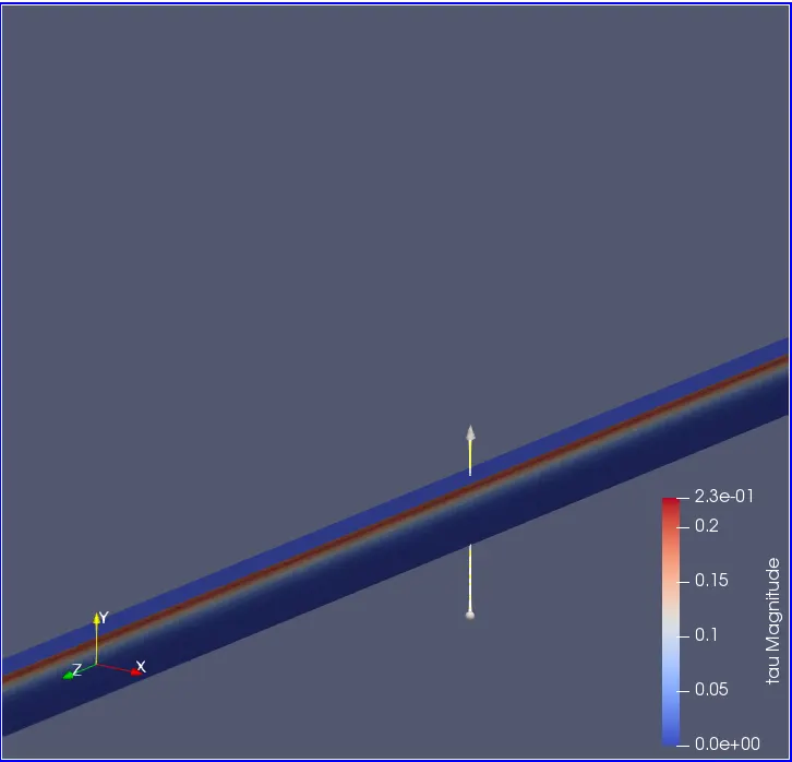
The line is drawn, as shown below:

Result:

1. The first simulation comparison is with the Wedge Boundary condition. Within this Boundary Condition, the simulation comparison for all the above-mentioned angles is as follows.
We will compare the Shear Stress developed for both the boundary conditions at all three angles.

a.Shear Stress Variation with respect to the Radial Distance.

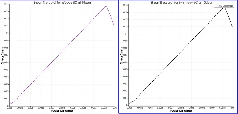
The Shear Stress plot for both the Boundary Conditions, the wedge Boundary Condition and the Symmetry Boundary Condition are shown at 10degrees. We can see that when we apply the Symmetry Boundary Condition, the slope of the curve is much higher than when we apply the Wedge Boundary Condition. So, when we apply the Symmetry Boundary Condition, the Mesh becomes 3D, and the computation is done for all three global axes. This affects the calculation as well. The peak value in the Wedge Boundary Condition is approximately 0.145 units, but whereas when we apply the Symmetry Boundary Condition, the peak value touches around 0.140units

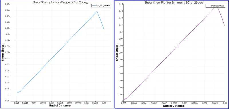
The graph shown above is comparing the Shear Stress for both the boundary conditions for when the wedge angle is 25degrees.

Similarly, we plot and study all the graphs, as shown below:

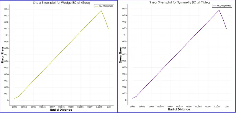
This graph compares the Shear Stress at 45 Deg for both the Boundary conditions.




b. Velocity Variation with respect to Radial Distance.

This graph compares the Shear Stress at 45 Deg for both the Boundary conditions.




b. Velocity Variation with respect to Radial Distance.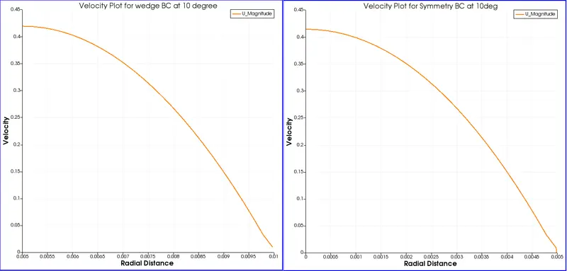


Velocity variation at 10degrees for the two Boundary Conditions.



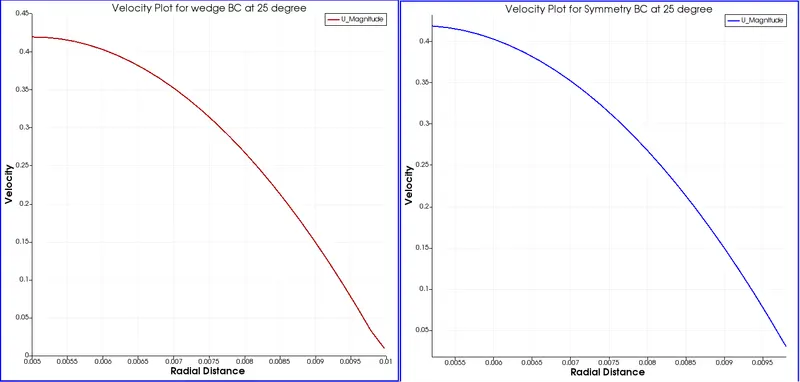
Velocity variation at 25 degrees for the two Boundary Conditions.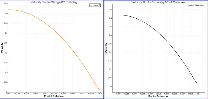

c. Pressure Drop across the axial Distance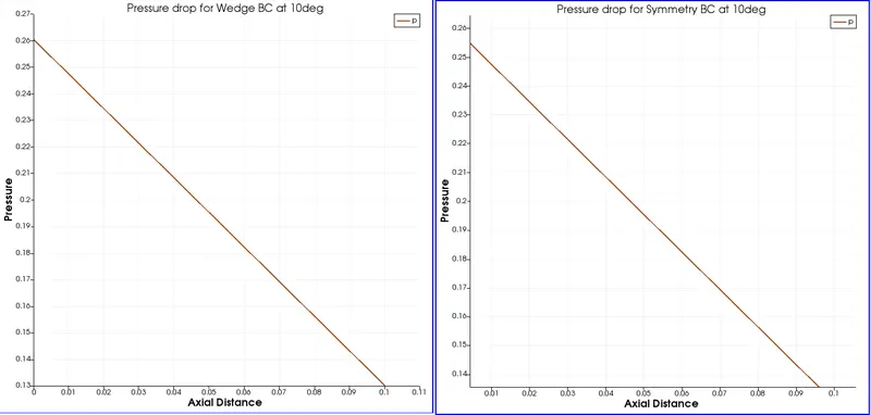


Pressure drop at 10 degrees across the Axial Distance.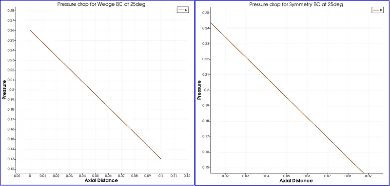




Pressure drop at 25 degrees across the Axial Distance.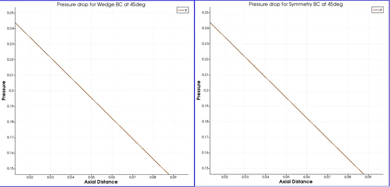




Pressure drop at 45 degrees across the Axial Distance.

c. Pressure Drop across the axial Distance

Pressure drop at 10 degrees across the Axial Distance.

Pressure drop at 25 degrees across the Axial Distance.

Pressure drop at 45 degrees across the Axial Distance.

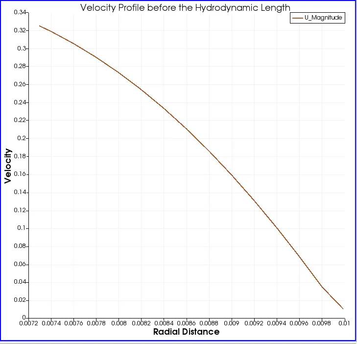
Whereas, if we compare the velocity profile at a location after the hydrodynamic length and in the fully developed region, the velocity profile will be much more defined and proper.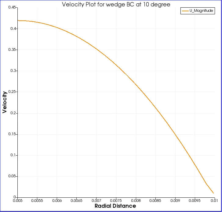

d. Shear Stress Plot: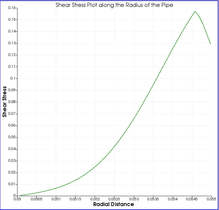

• Conclusion: In conclusion, I would like to state that this challenge helped me understand the difference between the two boundary conditions and how to simulate them as per the need of the problem that we will be simulating.