Challenge

Week 12 - Validation studies of Symmetry BC vs Wedge BC in OpenFOAM vs Analytical H.P equation

SShivranjan Jadhav31 Oct 2022

Week 12 -

Validation studies of Symmetry BC vs Wedge BC in OpenFOAM vs Analytical H.P equation

Question :

In this challenge you will simulate the same problem as in week 11 but by applying Symmetry Boundary Condition. You will do the simulation for the below mentioned angles using both symmetry and wedge boundary conditions and validate them with HP equations like you did in week 11 challenge.

Angles to test:

10⁰
25⁰
45⁰

Expected Results

Validate Hydro-dynamic length with the numerical result
Validate the fully developed flow velocity profile with its analytical profile
Validate maximum velocity and pressured drop for fully developed flow
Post-process Shear stress and validate wall shear stress for fully developed flow
Highligh the differences in both boundary conditions in terms of their usage and application.

Aim :

Simulate an axi-symmetric flow by applying the Symmetry boundary condition for a laminar flow through a constant cross-section pipe at an inlet Reynold's number of 2100.
Carry out transient or steady state simulation to validate the results with the Hagen- Poiseuille's equations for the fully developed flow.
To write a code in Matlab to automate the generation of blockMeshDict file, which takes inputs like pipe length, diameter, wedge angle, etc and outputs a fully functional blockMeshDict file. geometry.
Simulation for angle 10⁰, 20⁰, and 45⁰

Key Points :

Symmetry and Wedge Boundary Condition
Wedge Boundary Condition
Hagen- Poiseuille’s equation
Hydro-dynamic length
Comparison between results of Wedge and symmetry boundary conditions.

Symmetry Boundary Condition :-

This boundary condition is used to apply mirror-symmetry conditions to a structure.

It can be applied to the faces of a structure and no other user input is needed. If a symmetry plane condition is applied to a face, the displacement of this face is locked in a normal direction but free to slide in tangential directions.

During the time of numerical analysis, it calculates the flow field variables for the complete cell volume rather than taking a single plane as in Wedge BC.

The symmetry BC allows us to use multiple meshes keeping in mind the Courant number(more the meshes, lesser is the dx value), to be within the stability conditions.

For the Symmetry BC, the angular changes that are considered don't affect or create an unsteady pattern for the path of attaining the convergence.

Wedge Boundary Condition :-

Wedge means ' taking small portion of entire object.

The wedge boundary condition is used in computational fluid dynamics to define an axisymmetric situation, for eg. a cylinder. The model and flow must be axisymmetric along a central line such that all physical variables of the flow have the same value and distribution at a given radius for all angles.

This boundary condition is specified by two planes that must be selected on separate sides of the domain (referred to as front and back) on surfaces running along the axis. It works for 2D simulations only.

A Wedge boundary is different from the symmetry boundary condition in the sense that the wedge boundary condition applies the Navier-Stokes (NS) equations in cylindrical coordinates whereas the symmetric applies the NS equations in cartesian coordinates. One big advantage of wedge boundary is that it allows for the rotational flow around the axis and this is possible only because the fluxes and normal components are not assumed as zero.

The wedge BC considers only a single straight mid-plane for a given wedge-shaped geometry(the triangular kind of looking shape) and represents the simulated values of the flow field variables only through that plane. The plane looks like when it is rotated 360 degrees it forms a full cylinder.

Usage of Wedge BC limits our input value of a number of meshes along the wedge. Usage of many meshes in Wedge BC leads to errors in the result.

Hagen- Poiseuille's Theory :-

In nonideal fluid dynamics, the Hagen–Poiseuille equation, also known as the Hagen–Poiseuille law, Poiseuille law or Poiseuille equation, is a physical law that gives the pressure drop in an incompressible and Newtonian fluid in laminar flow flowing through a long cylindrical pipe of constant cross section.

The assumptions of the equation are that the fluid is incompressible and Newtonian; the flow is laminar through a pipe of constant circular cross-section that is substantially longer than its diameter; and there is no acceleration of fluid in the pipe. The pressure drop in an incompressible and Newtonian fluid in laminar flow through a long cylindrical pipe of constant cross – section can be derived as,

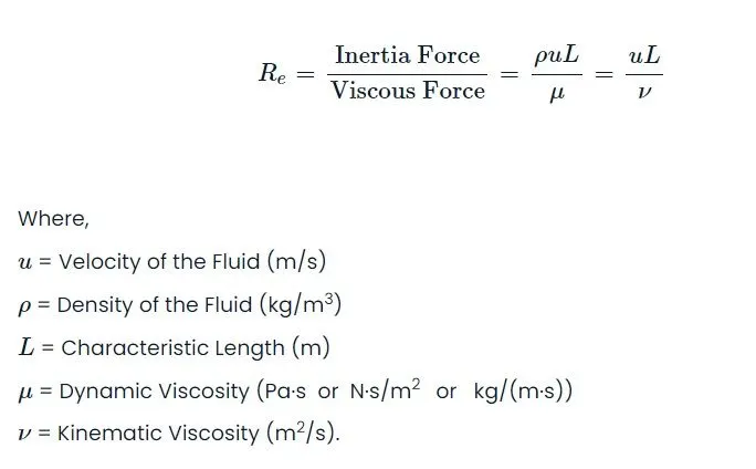
The ratio of length to radius of a pipe should be greater than one forty-eighth of the Reynolds number for the Hagen–Poiseuille law to be valid. If the pipe is too short, the Hagen–Poiseuille equation may result in unphysically high flow rates.

A few examples in which the Hagen–Poiseuille law is practically applied is the air flow in lung alveoli, or the flow through a drinking straw or through a hypodermic needle. It is also applied for the process of blood flow through a narrow constriction.

Hydro-dynamic length :-

In fluid dynamics, the entrance length is the distance a flow travels after entering a pipe before the flow becomes fully developed.

Entrance length refers to the length of the entry region, the area following the pipe entrance where effects originating from the interior wall of the pipe propagate into the flow as an expanding boundary layer. When the boundary layer expands to fill the entire pipe, the developing flow becomes a fully developed flow, where flow characteristics no longer change with increased distance along the pipe. Many different entrance lengths exist to describe a variety of flow conditions.

Hydrodynamic entrance length describes the formation of a velocity profile caused by viscous forces propagating from the pipe wall. Thermal entrance length describes the formation of a temperature profile. Awareness of entrance length may be necessary for the effective placement of instrumentation, such as fluid flow meters.

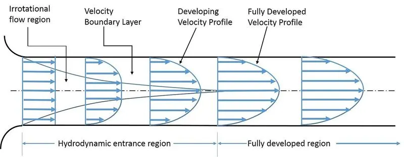
The hydrodynamic entrance region refers to the area of a pipe where fluid entering a pipe develops a velocity profile due to viscous forces propagating from the interior wall of a pipe. This region is characterized by a non-uniform flow. The fluid enters a pipe at a uniform velocity, then fluid particles in the layer in contact with the surface of the pipe come to a complete stop due to the no-slip condition. Due to viscous forces within the fluid, the layer in contact with the pipe surface resists the motion of adjacent layers and slows adjacent layers of fluid down gradually, forming a velocity profile. For the conservation of mass to hold true, the velocity of layers of the fluid in the center of the pipe increases to compensate for the reduced velocities of the layers of fluid near the pipe surface. This develops a velocity gradient across the cross-section of the pipe.

Shear Stress :-

In the hydrodynamic entrance region, the wall shear stress (τw ) is highest at the pipe inlet, where the boundary layer thickness is the smallest. Shear stress decreases along the flow direction. That is why the pressure drop is highest in the entrance region of a pipe, which increases the average friction factor for the whole pipe. This increase in the friction factor is negligible for long pipes.
In a fully developed region, the pressure gradient and the shear stress in flow are in balance.

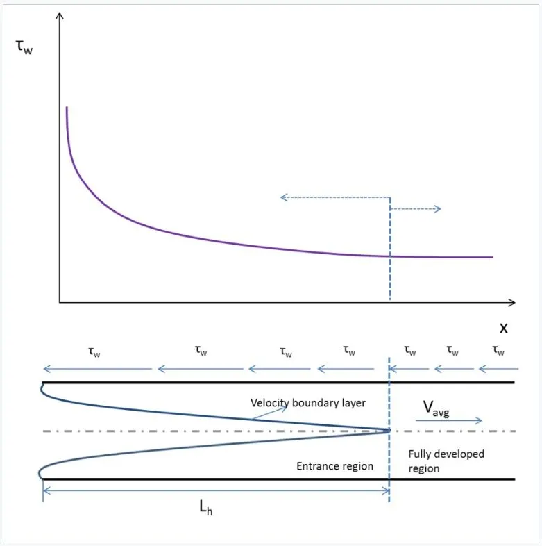
Now consider flow through circular pipe with uniform velocity,

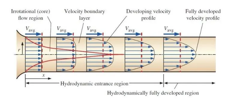
As a result of the no-slip conditions along the walls of the pipe, the fluid particles that come in contact with the wall come to a complete stop. As a result of friction, this causes the adjacent layers of the fluid to slow down as well. To make up for the reduction in velocity, the fluid velocity at the mid-section of the pipe has to increase to maintain a constant mass flow rate through the pipe.

The various regions of the pipe as shown in the above diagram are as follows,

The irrotational (core) flow region is one in which the frictional effects are negligible and the velocity remains essentially constant in the radial direction.
The region of flow in which the effects of viscous shearing forces caused by fluid viscosity are felt and the velocity changes are significant, is referred to as the velocity boundary layer.
The region from the pipe inlet to the point at which the velocity profile is fully developed is called the hydrodynamic entrance region and the length of this region is referred to as the hydrodynamic entry length.
Flow in the entrance region is called hydrodynamically developing flow since it is where the velocity profile develops. The region beyond the entrance region in which the velocity profile is fully developed and remains unchanged is called the hydrodynamically fully developed region.

Given Data :

Geometry of the flow is axi - symmetric.

The flow is laminar and flows through a constant cross section.

Inlet Reynold’s Number,

Re = 2100

Angle 10⁰, 25⁰ and 45⁰.

Analytical Solution : -

Diameter of Pipe :-

D = 0.02 m

R = D/2 = 0.01m

Density of fluid (Water) : -

ρ = 997 kg/m^3

Wedge Angle : - Ɵ = 10⁰.

Dynamic Viscosity of water at 25⁰C

`mu = 8.90 xx 10^-4 Pa.s`

Kinematic Viscosity of water at 25⁰C

ν = µ / ρ = (8.90 x 10^-4) / 997

ν = 8.92 X 10 ^-7 m^2/s

Hydrodynamic Entrance Length :-

Lh = 0.06 . Re . D = 0.06 x 2100 x 0.02

Lh = 2.52m

Total Length of pipe :-

L = 2.8m

Average Velocity :-

Vavg = (µ . Re) / (ρ . D) = 0.0937 m/s

Maximum Velocity :-

Vmax = 2 . Vavg = 0.1874 m/s

Velocity Profile :-

`μ(r)=2⋅V_(avg)⋅(1-γ^2/R^2 )`

Pressure drop :-

`ΔP=(32⋅μ⋅V_(avg)⋅L)/D^2`

`ΔP=(32 xx 8.90 xx 10^(-4) xx 0.0937xx 2.8)/(0.02)^2`

`ΔP=18.680 Pa`

Kinematic pressure drop :-

`sf "Kinematic" Δp= (ΔP)/ρ=18.680/997`

`sf "Kinematic" Δp= 0.0187 Pa`

Shear stress :-

`τ=(2⋅μ⋅V_max⋅R_e)/R^2`

`τ=(2 xx 8.90 xx 10^(-4) xx 0.1874 xx 2100)/0.01^2`

`τ=7005.012 Pa`

Task 1: create an matlab script whcih can create an blockmeshdict file automatically for various values of the wedge angle

SIMULATION PROCEDURE :

Problem Setup :

We first initialize the problem by navigating to the tutorials directory of OpenFOAM by using the “tut” command in the terminal window.
From the tutorials, we have to figure out the suitable case file for our given problem, which is an axi-symmetric laminar flow through a constant cross section pipe. We use the “ls” command to list the contents (files or directories) present inside the directory..
As it is an incompressible flow, we navigate into the incompressible directory. We use the “cd” command to navigate and change the working directory using the terminal window.
The next step involves navigating into the icoFoam directory, as the type of solver for this problem is icoFoam. The icoFoam command solves the incompressible laminar Navier-Stokes equations. The code is inherently transient, requiring an initial condition (such as zero velocity) and boundary conditions.
Here, we use the cavity utility to create our required domain. We copy this directory into the $FOAM_RUN file, which is a default file OpenFOAM creates for us. We use the “cp -r” command to recursively create a copy of the contents of the file or directory into the $FOAM_RUN folder under the file name “Pipe_BC”, for personal use. We create a copy of the files as OpenFOAM does not let us modify or make changes to its inbuilt tutorial files.
We then navigate to the copied tutorial file in the $FOAM_RUN directory to view the contents inside the folder.

Creating Geometry for Wedge Boundary condition:-

In order to fully take the advantage of the symmetry involved in the geometry we use the type called as wedge in the geometry. The cyclinder/pipe is divided along its axis since the flow in this case is axisymmetric. The angle of the cut used is 4 degrees. The geometry developed and the node nomenclature used is as follows:

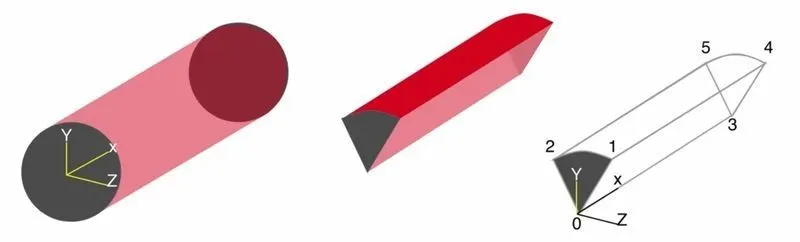
Case 1: Wedge boundary condition with angle 10⁰

Matlab code to create blockMeshDict for Wedge boundary condition with angle 10⁰:-

clear
close
clc
 
%% INPUTS
% Diameter of Pipe (m)
D = 0.02; 
 
% Radius of Pipe (m)
R = D/2;
 
% Reynold's Number
Re = 2100;
 
% Wedge Angle (degrees)
theta = 10;
 
% Total Length of the Pipe (m)
L = 2.8;
 
 
 
% Assuming working fluid is water at 25° C
% Density of water (kg/m³)
rho = 997;
 
% Dynamic Viscosity of Water (Pa.s)
mu = 8.90 * 10^-4;
 
% Kinematic Viscosity of Water (m^2/s)
nu = mu/rho;
 
 
% Hydrodynamic Entrance Length (m)
L_h = 0.06 * Re * D;
 
 
 
%% HAGEN - POISEUILLE'S FLOW EQUATIONS
% Average Velocity (m/s)
V_avg = (mu * Re)/(rho * D);
 
% Maximum Velocity (m/s)
V_max = 2 * V_avg;
 
% Pressure Drop (Pa)
delta_p = (32*mu*V_avg*L)/(D^2);
 
% Kinematic Pressure Drop (Pa)
kinematic_delta_p = delta_p/rho;
 
%% Calculating shear stress
r = linspace(0,(D/2),500);
for i = 1:length(r)
    tau(i) = 2 * mu * V_max * abs(r(i))/R^2;
end
figure(1)
 
plot(r,tau)
 
xlabel('Radius of pipe')
 
ylabel('shear stress')
 
title('shear stress')
 
legend('shear stress')

 
 
%% DEFINING THE GEOMETRY
% Vertices
V0 = [0 0 0];
V1 = [0 R*cosd(theta/2) -R*sind(theta/2)];
V2 = [0 R*cosd(theta/2) R*sind(theta/2)];
 
V3 = [L 0 0];
V4 = [L R*cosd(theta/2) -R*sind(theta/2)];
V5 = [L R*cosd(theta/2) R*sind(theta/2)];
 
 
%% BLOCKMESHDICT FILE
% Creating the file
% Header
h1 = '/*--------------------------------*- C++ -*----------------------------------*\';
h2 = '  =========                 |';
h3 = '  \\      /  F ield         | OpenFOAM: The Open Source CFD Toolbox';
h4 = '   \\    /   O peration     | Website:  https://openfoam.org';
h5 = '    \\  /    A nd           | Version:  9';
h6 = '     \\/     M anipulation  |';
h7 = '\*---------------------------------------------------------------------------*/';
h8 = 'FoamFile';
h9 = '{';
h10 = '    format      ascii;';
h11 = '    class       dictionary;';
h12 = '    object      blockMeshDict;';
h13 = '}';
h14 = '// * * * * * * * * * * * * * * * * * * * * * * * * * * * * * * * * * * * * * //';
 
 
%% Creating BlockMesh File
f1 = fopen('blockMeshDict.txt','w');
 
% Header
fprintf(f1,'%s\n',h1);
fprintf(f1,'%s\n',h2);
fprintf(f1,'%s\n',h3);
fprintf(f1,'%s\n',h4);
fprintf(f1,'%s\n',h5);
fprintf(f1,'%s\n',h6);
fprintf(f1,'%s\n',h7);
fprintf(f1,'%s\n',h8);
fprintf(f1,'%s\n',h9);
fprintf(f1,'%s\n',h10);
fprintf(f1,'%s\n',h11);
fprintf(f1,'%s\n',h12);
fprintf(f1,'%s\n',h13);
fprintf(f1,'%s\n\n',h14);
 
% Conversion Factor
fprintf(f1,'%s\n\n','convertToMeters 1;');
 
% Vertices
fprintf(f1,'%s\n','vertices');
fprintf(f1,'%s\n','(');
fprintf(f1,'\t(%d %d %d)\n',V0);
fprintf(f1,'\t(%d %f %f)\n',V1);
fprintf(f1,'\t(%d %f %f)\n',V2);
fprintf(f1,'\t(%.2f %d %d)\n',V3);
fprintf(f1,'\t(%.2f %f %f)\n',V4);
fprintf(f1,'\t(%.2f %f %f)\n',V5);
fprintf(f1,'%s\n\n',');');
 
% Blocks
fprintf(f1,'%s\n','blocks');
fprintf(f1,'%s\n','(');
fprintf(f1,'\thex (0 3 4 1 0 3 5 2) (400 30 1) simpleGrading (1 0.1 1)\n');
fprintf(f1,'%s\n\n',');');
 
% Edges
fprintf(f1,'%s\n','edges');
fprintf(f1,'%s\n','(');
fprintf(f1,'\tarc 2 1 (%d %.3f %d)\n',0,R,0);
fprintf(f1,'\tarc 5 4 (%.3f %.3f %d)\n',L,R,0);
fprintf(f1,'%s\n\n',');');
 
% Boundary
fprintf(f1,'%s\n','boundary');
fprintf(f1,'%s\n','(');
 
% Axis
fprintf(f1,'\taxis\n');
fprintf(f1,'\t{\n');
fprintf(f1,'\t\ttype empty;\n');
fprintf(f1,'\t\tfaces\n');
fprintf(f1,'\t\t(\n');
fprintf(f1,'\t\t\t(0 3 3 0)\n');
fprintf(f1,'\t\t);\n');
fprintf(f1,'\t}\n\n');
 
% Inlet
fprintf(f1,'\tinlet\n');
fprintf(f1,'\t{\n');
fprintf(f1,'\t\ttype patch;\n');
fprintf(f1,'\t\tfaces\n');
fprintf(f1,'\t\t(\n');
fprintf(f1,'\t\t\t(0 1 2 0)\n');
fprintf(f1,'\t\t);\n');
fprintf(f1,'\t}\n\n');
 
% Outlet
fprintf(f1,'\toutlet\n');
fprintf(f1,'\t{\n');
fprintf(f1,'\t\ttype patch;\n');
fprintf(f1,'\t\tfaces\n');
fprintf(f1,'\t\t(\n');
fprintf(f1,'\t\t\t(3 5 4 3)\n');
fprintf(f1,'\t\t);\n');
fprintf(f1,'\t}\n\n');
 
% Front Face
fprintf(f1,'\tfront\n');
fprintf(f1,'\t{\n');
fprintf(f1,'\t\ttype wedge;\n');
fprintf(f1,'\t\tfaces\n');
fprintf(f1,'\t\t(\n');
fprintf(f1,'\t\t\t(0 3 4 1)\n');
fprintf(f1,'\t\t);\n');
fprintf(f1,'\t}\n\n');
 
% Back Face
fprintf(f1,'\tback\n');
fprintf(f1,'\t{\n');
fprintf(f1,'\t\ttype wedge;\n');
fprintf(f1,'\t\tfaces\n');
fprintf(f1,'\t\t(\n');
fprintf(f1,'\t\t\t(0 2 5 3)\n');
fprintf(f1,'\t\t);\n');
fprintf(f1,'\t}\n\n');
 
% Top Wall
fprintf(f1,'\tpipeWall\n');
fprintf(f1,'\t{\n');
fprintf(f1,'\t\ttype wall;\n');
fprintf(f1,'\t\tfaces\n');
fprintf(f1,'\t\t(\n');
fprintf(f1,'\t\t\t(1 4 5 2)\n');
fprintf(f1,'\t\t);\n');
fprintf(f1,'\t}\n');
 
fprintf(f1,'%s\n\n',');');
fprintf(f1,'%s\n','mergePatchPairs');
fprintf(f1,'%s\n','(');
fprintf(f1,'%s\n\n',');');
fprintf(f1,'%s\n','// ************************************************************************* //');

Output of MATLAB code :-

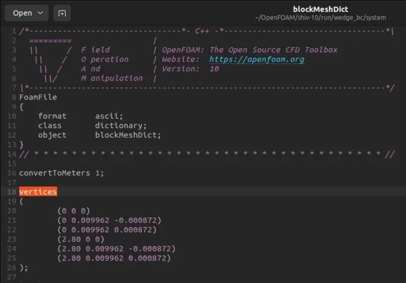
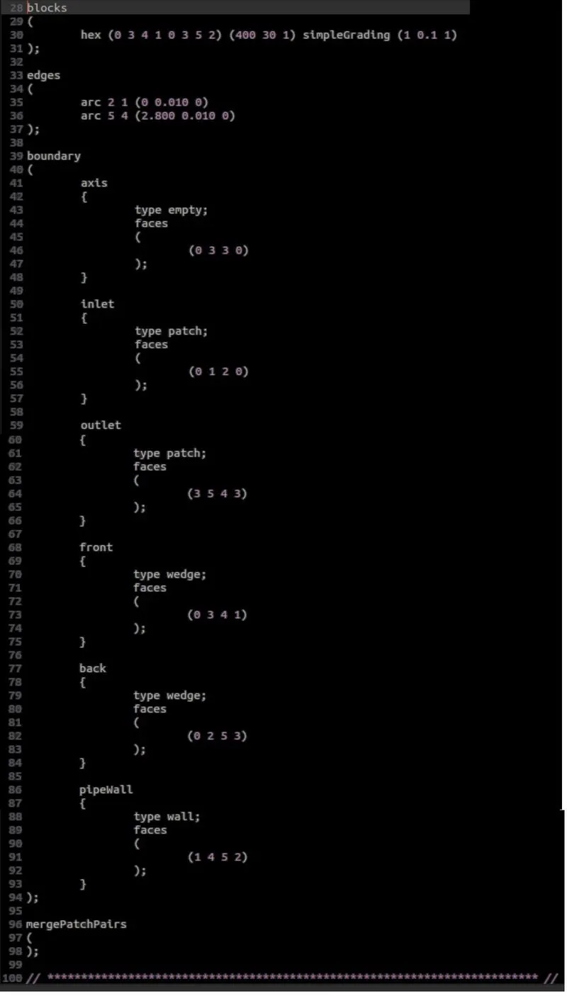
BlockMeshDict file for Wedge boundary condition with angle 10⁰:-

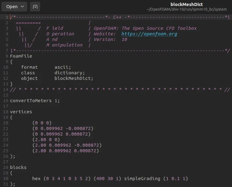
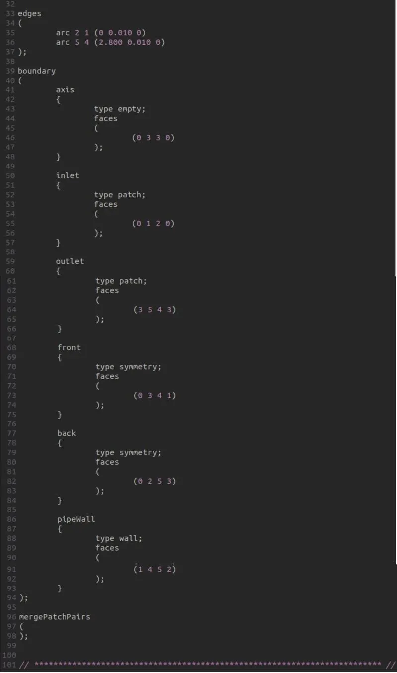
The blockMeshDict file has been written automatically by the MatLab program as shown above, which we use to create the geometry of the wedge and run the simulation for the same.

ControlDict file :-

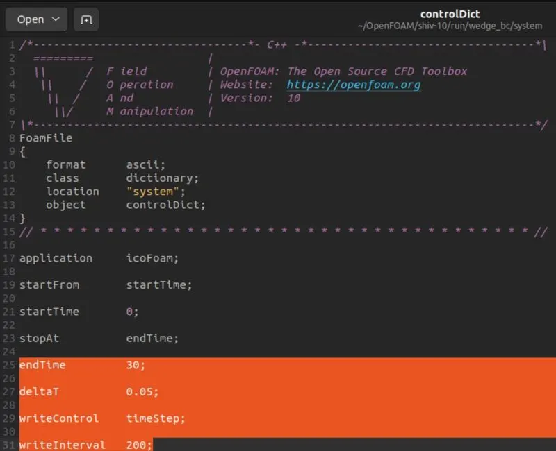
In controlDict file we will change End Time, Delta T and Write Interval values.

End Time :- To decide suitable end time we will first decide minimum time required to run simulation by formula Velocity = Dist / Time

Time required = Total length / Avg velocity

= 2.8/0.0937 =29.88 Sec

So, we will put value of end time 30 Sec

Delta T :- We will check for 0.01 if found error we will change value according to required number of Iterations to solve.
- In this case for Delta T = 0.01 it took so much time to run so we will change Delta T = 0.05

Write Interval :- This defines time after which new interval decides and new folder created for that each interval. So if interval value is less, solver take so many intervals so we will increase value accordingly.
- In this case for Write Interval = 20, it took so many interval to run so we will change Write Interval = 200

We did not make any other changes in ControlDict file and save it.

We will not change in any remaining part in ControlDict file

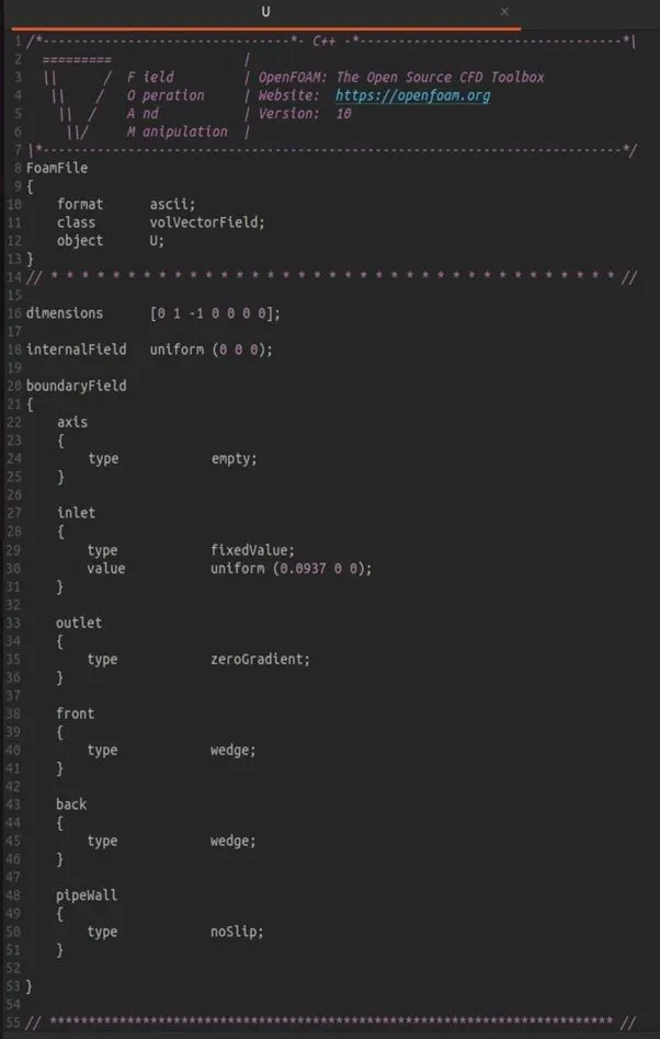
U file (Velocity) :-

We will make changes in velocity file located in

“0” folder --> U file

We will make changes in boundary field and use same names for boundary fields as used in BlockMeshDict file.

We also define type of boundary field as per geometry.

Boundary	Type	Discreption
Axis	empty	Empty Patch field
Inlet	fixedValue	Predefining values of variables
Outlet	zeroGradient	All variable are set to constant
Front	wedge	define an axisymmetric situation
Back	wedge	define an axisymmetric situation
PipeWall	noSlip	No slip in velocity at wall

After changing all boundary fields and type we will change value of Inlet for velocity. We are considering average velocity of fluid at inlet so change type of inlet to fixedValue and change value of inlet to 0.0937 in X-direction.

P file (Pressure) :-

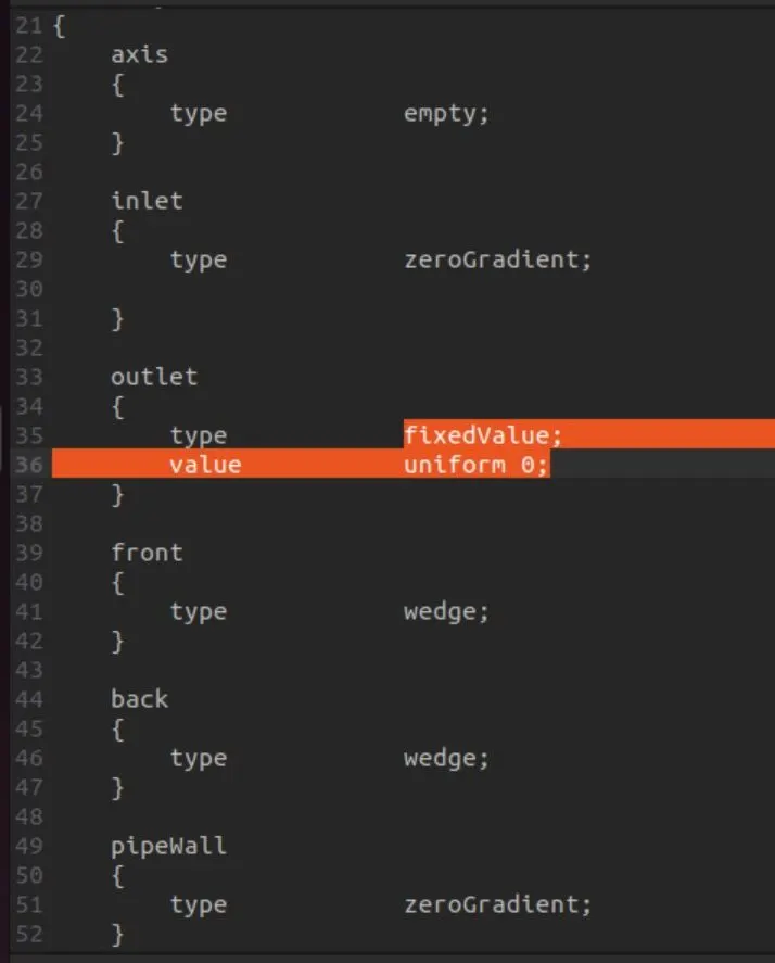
Pressure file located in “0” folder --> P file

We will change in boundary fields as done in Velocity file only difference is that we are not using predefined value for pressure at inlet. We are keeping pressure constant at inlet and changing value of pressure to zero at outlet as shown below.

Physical Properties file :-

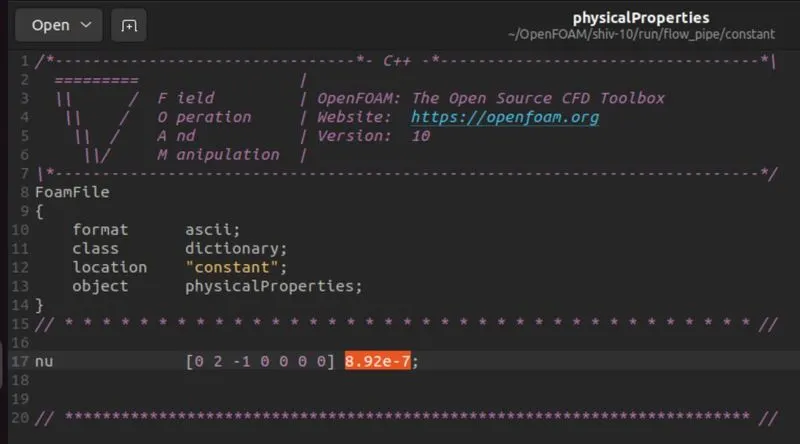
Located in “Constant” folder --> physicalProperties file

As we are considering water as fluid at 25⁰ C so We will change value of kinematic viscosity to 8.92e-7 i.e. (8.92 x 10^-7)

Now after saving all these changes in editor, we will create Mesh in OpenFoam by running blockMesh command in
After running blockMesh successfully we will run icoFoam command in terminal.
After completing all iterations we will run touch command to create and save Paraview model file with “name.foam” extension.
For this case : “touch wedge_10.foam”
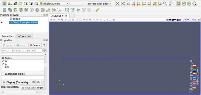
Now we will run paraFoam command to see ParaView of model.

ParaView of model :

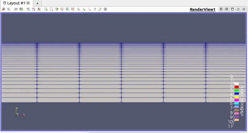
Detailed View :-

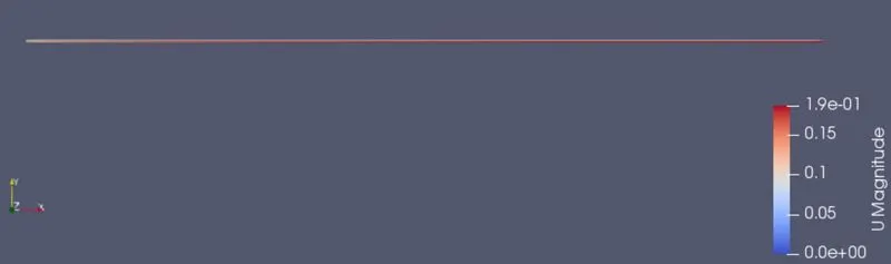
Velocity Distribution :-

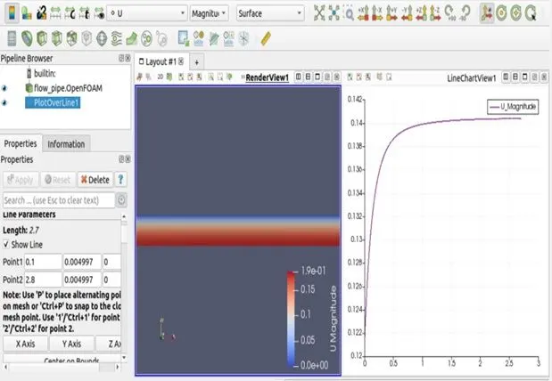
Velocity Profile :-

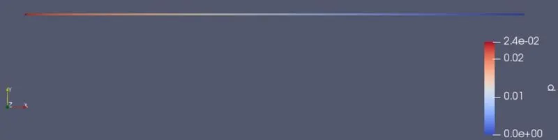
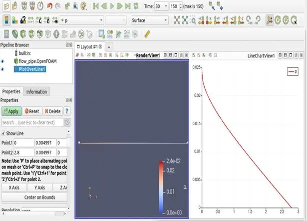
Pressure Distribution :-

Pressure Profile :-

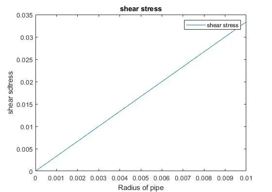
Graph of Shear Stress distribution from MatLab:-

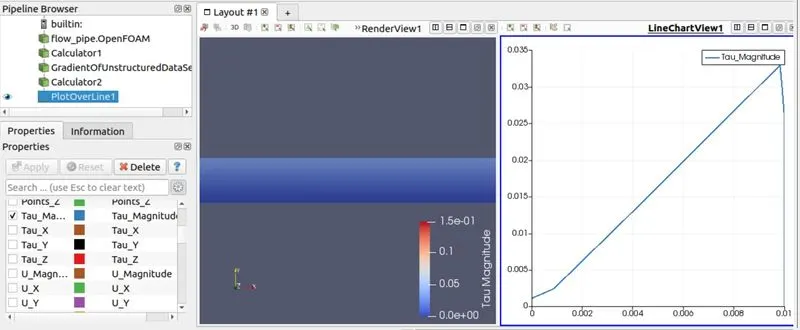
Shear Stress distribution in ParaView :-

Wedge Boundary condition with angle 25⁰ :-

For 25⁰ angle, we will copy entire folder created for wedge boundary condition with 10⁰ angle including Matlab code.

We will make changes in Matlab code created for 10⁰ and change value of theta to 25 from 10, as shown below.

clear
close
clc
 
%% INPUTS
% Diameter of Pipe (m)
D = 0.02; 
 
% Radius of Pipe (m)
R = D/2;
 
% Reynold's Number
Re = 2100;
 
% Wedge Angle (degrees)
theta = 25;
 
% Total Length of the Pipe (m)
L = 2.8;

We will not make any other changes in remaining code.

Due to changing in theta value, vertices will change in output BlockMeshDict file.

For wedge boundary condition with 25⁰ , we will change only vertices and no other change is necessary.

No need to make any changes in ControlDict, pressure, velocity and physical property file for same boundary condition.

Similarly, we follow same procedure for wedge boundary condition with angle 45⁰

ParaView Model for Wedge Bondary condition :-

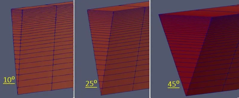
Case 2

Symmetry Boundary condition with angle 10⁰ :-

For symmetry boundary condition with 10⁰ angle, we will copy folder created for wedge boundary with 10⁰ angle. We will edit Matlab code and change boundary conditions for front face and back face to Symmetry as shown below

clear
close
clc
 
%% INPUTS
% Diameter of Pipe (m)
D = 0.02; 
 
% Radius of Pipe (m)
R = D/2;
 
% Reynold's Number
Re = 2100;
 
% Wedge Angle (degrees)
theta = 10;
 
% Total Length of the Pipe (m)
L = 2.8;
 
 
 
% Assuming working fluid is water at 25° C
% Density of water (kg/m³)
rho = 997;
 
% Dynamic Viscosity of Water (Pa.s)
mu = 8.90 * 10^-4;
 
% Kinematic Viscosity of Water (m^2/s)
nu = mu/rho;
 
 
% Hydrodynamic Entrance Length (m)
L_h = 0.06 * Re * D;
 
 
 
%% HAGEN - POISEUILLE'S FLOW EQUATIONS
% Average Velocity (m/s)
V_avg = (mu * Re)/(rho * D);
 
% Maximum Velocity (m/s)
V_max = 2 * V_avg;
 
% Pressure Drop (Pa)
delta_p = (32*mu*V_avg*L)/(D^2);
 
% Kinematic Pressure Drop (Pa)
kinematic_delta_p = delta_p/rho;
 
 
%% Calculating shear stress
r = linspace(0,(D/2),500);
for i = 1:length(r)
    tau(i) = 2 * mu * V_max * abs(r(i))/R^2;
end
figure(1)
 
plot(r,tau)
 
xlabel('Radius of pipe')
 
ylabel('shear stress')
 
title('Shear stress for Symmetry Boundary condition with angle 10?')
 
legend('shear stress')
 
%% DEFINING THE GEOMETRY
% Vertices
V0 = [0 0 0];
V1 = [0 R*cosd(theta/2) -R*sind(theta/2)];
V2 = [0 R*cosd(theta/2) R*sind(theta/2)];
 
V3 = [L 0 0];
V4 = [L R*cosd(theta/2) -R*sind(theta/2)];
V5 = [L R*cosd(theta/2) R*sind(theta/2)];
 
 
 
 
%% BLOCKMESHDICT FILE
% Creating the file
% Header
h1 = '/*--------------------------------*- C++ -*----------------------------------*\';
h2 = '  =========                 |';
h3 = '  \\      /  F ield         | OpenFOAM: The Open Source CFD Toolbox';
h4 = '   \\    /   O peration     | Website:  https://openfoam.org';
h5 = '    \\  /    A nd           | Version:  9';
h6 = '     \\/     M anipulation  |';
h7 = '\*---------------------------------------------------------------------------*/';
h8 = 'FoamFile';
h9 = '{';
h10 = '    format      ascii;';
h11 = '    class       dictionary;';
h12 = '    object      blockMeshDict;';
h13 = '}';
h14 = '// * * * * * * * * * * * * * * * * * * * * * * * * * * * * * * * * * * * * * //';
 
 
%% Creating BlockMesh File
f1 = fopen('blockMeshDictS10.txt','w');
 
% Header
fprintf(f1,'%s\n',h1);
fprintf(f1,'%s\n',h2);
fprintf(f1,'%s\n',h3);
fprintf(f1,'%s\n',h4);
fprintf(f1,'%s\n',h5);
fprintf(f1,'%s\n',h6);
fprintf(f1,'%s\n',h7);
fprintf(f1,'%s\n',h8);
fprintf(f1,'%s\n',h9);
fprintf(f1,'%s\n',h10);
fprintf(f1,'%s\n',h11);
fprintf(f1,'%s\n',h12);
fprintf(f1,'%s\n',h13);
fprintf(f1,'%s\n\n',h14);
 
% Conversion Factor
fprintf(f1,'%s\n\n','convertToMeters 1;');
 
% Vertices
fprintf(f1,'%s\n','vertices');
fprintf(f1,'%s\n','(');
fprintf(f1,'\t(%d %d %d)\n',V0);
fprintf(f1,'\t(%d %f %f)\n',V1);
fprintf(f1,'\t(%d %f %f)\n',V2);
fprintf(f1,'\t(%.2f %d %d)\n',V3);
fprintf(f1,'\t(%.2f %f %f)\n',V4);
fprintf(f1,'\t(%.2f %f %f)\n',V5);
fprintf(f1,'%s\n\n',');');
 
% Blocks
fprintf(f1,'%s\n','blocks');
fprintf(f1,'%s\n','(');
fprintf(f1,'\thex (0 3 4 1 0 3 5 2) (400 30 1) simpleGrading (1 0.1 1)\n');
fprintf(f1,'%s\n\n',');');
 
% Edges
fprintf(f1,'%s\n','edges');
fprintf(f1,'%s\n','(');
fprintf(f1,'\tarc 2 1 (%d %.3f %d)\n',0,R,0);
fprintf(f1,'\tarc 5 4 (%.3f %.3f %d)\n',L,R,0);
fprintf(f1,'%s\n\n',');');
 
% Boundary
fprintf(f1,'%s\n','boundary');
fprintf(f1,'%s\n','(');
 
% Axis
fprintf(f1,'\taxis\n');
fprintf(f1,'\t{\n');
fprintf(f1,'\t\ttype empty;\n');
fprintf(f1,'\t\tfaces\n');
fprintf(f1,'\t\t(\n');
fprintf(f1,'\t\t\t(0 3 3 0)\n');
fprintf(f1,'\t\t);\n');
fprintf(f1,'\t}\n\n');
 
% Inlet
fprintf(f1,'\tinlet\n');
fprintf(f1,'\t{\n');
fprintf(f1,'\t\ttype patch;\n');
fprintf(f1,'\t\tfaces\n');
fprintf(f1,'\t\t(\n');
fprintf(f1,'\t\t\t(0 1 2 0)\n');
fprintf(f1,'\t\t);\n');
fprintf(f1,'\t}\n\n');
 
% Outlet
fprintf(f1,'\toutlet\n');
fprintf(f1,'\t{\n');
fprintf(f1,'\t\ttype patch;\n');
fprintf(f1,'\t\tfaces\n');
fprintf(f1,'\t\t(\n');
fprintf(f1,'\t\t\t(3 5 4 3)\n');
fprintf(f1,'\t\t);\n');
fprintf(f1,'\t}\n\n');
 
% Front Face
fprintf(f1,'\tfront\n');
fprintf(f1,'\t{\n');
fprintf(f1,'\t\ttype symmetry;\n');
fprintf(f1,'\t\tfaces\n');
fprintf(f1,'\t\t(\n');
fprintf(f1,'\t\t\t(0 3 4 1)\n');
fprintf(f1,'\t\t);\n');
fprintf(f1,'\t}\n\n');
 
% Back Face
fprintf(f1,'\tback\n');
fprintf(f1,'\t{\n');
fprintf(f1,'\t\ttype symmetry;\n');
fprintf(f1,'\t\tfaces\n');
fprintf(f1,'\t\t(\n');
fprintf(f1,'\t\t\t(0 2 5 3)\n');
fprintf(f1,'\t\t);\n');
fprintf(f1,'\t}\n\n');
 
% Top Wall
fprintf(f1,'\tpipeWall\n');
fprintf(f1,'\t{\n');
fprintf(f1,'\t\ttype wall;\n');
fprintf(f1,'\t\tfaces\n');
fprintf(f1,'\t\t(\n');
fprintf(f1,'\t\t\t(1 4 5 2)\n');
fprintf(f1,'\t\t);\n');
fprintf(f1,'\t}\n');
 
fprintf(f1,'%s\n\n',');');
fprintf(f1,'%s\n','mergePatchPairs');
fprintf(f1,'%s\n','(');
fprintf(f1,'%s\n\n',');');
fprintf(f1,'%s\n','// ************************************************************************* //');

BlockMeshDict file for Symmetry boundary condition with angle 10⁰:-

ControlDict file for Symmetry BC with 10⁰:-

In controlDict file we will kept End Time, Delta T and Write Interval values same as used for wedge boundary conditions. We will not make any changes.

U file (Velocity) and p file (Pressure) :-

We will make changes in velocity and pressure file located in

“0” folder à U file and P file

We will make changes in boundary field and use same names for boundary fields as used in BlockMeshDict file.

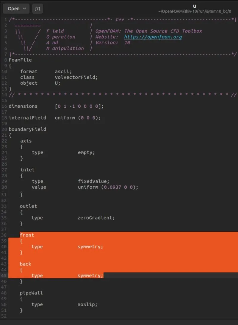
We also define type of boundary field for front and back faces type to “symmetry” from “wedge” as shown below.

No need to change anything else except front and back face type.

We will kept physicalProperties file same as used for previous case.

Symmetry Boundary condition with angle 25⁰ :-

For 25⁰ angle, we will copy entire folder created for symmetry boundary condition with 10⁰ angle including Matlab code.

We will make changes in Matlab code created for 10⁰ and change value of theta to 25 from 10, as shown below.

clear
close
clc
 
%% INPUTS
% Diameter of Pipe (m)
D = 0.02; 
 
% Radius of Pipe (m)
R = D/2;
 
% Reynold's Number
Re = 2100;
 
% Wedge Angle (degrees)
theta = 25;
 
% Total Length of the Pipe (m)
L = 2.8;

We will not make any other changes in remaining code.

Due to changing in theta value, vertices will change in output BlockMeshDict file.

For symmetry boundary condition with 25⁰ , we will change only vertices and no other change is necessary.

No need to make any changes in ControlDict, pressure, velocity and physical property file for same boundary condition.

Similarly, we follow same procedure for symmetry boundary condition with angle 45⁰

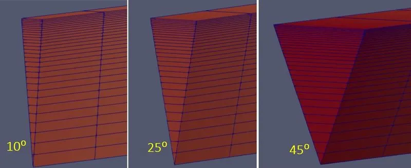
ParaView Model for Symmetry Bondary condition :-

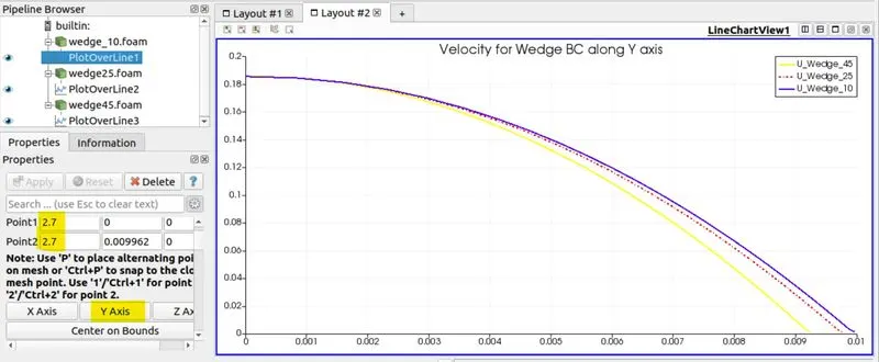
Velocity profile for Wedge BC along Y axis :- (Vmax)

Velocity profile for Symmetry BC along Y axis :- (Vmax)

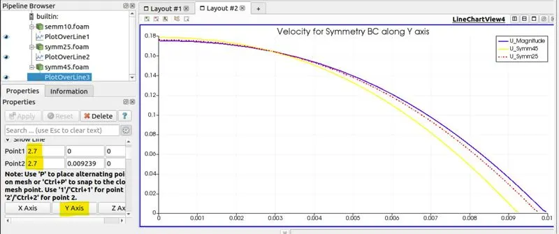
Comparison of Analytical values and CFD simulation values :-

Average Velocity = 2 x Max. Velocity

Pressure drop in CFD simulation for wedge BC :-

`ΔP=(32⋅μ⋅V_(avg)⋅L)/D^2`

`ΔP=(32 xx 8.90 xx 10^(-4) xx 0.0928 xx 2.8)/(0.02)^2`

`ΔP=18.500 Pa`

Term	Analytical Value	Simulation Value
Max Velocity	0.1874 m/s	0.1856 m/s
Avg Velocity	0.0937 m/s	0.0928 m/s
Hydro dynamic length	2.52 m	2.3 m
Pressure Drop	18.680 Pa	18.5 Pa

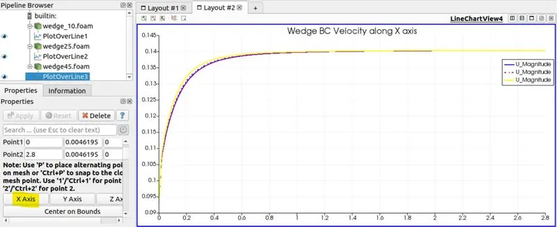
Comparison of Velocity profile for Wedge Boundary conditions at different angles :-

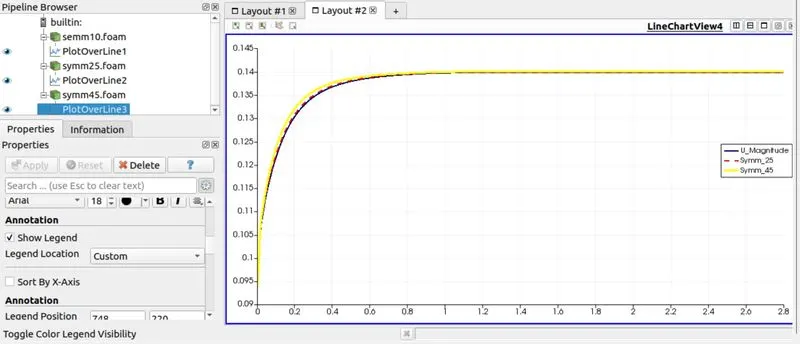
Comparison of Velocity profile for Symmetry Boundary conditions at different angles :-

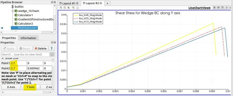
Comparison of Shear stress distribution for Wedge Boundary conditions at different angles :-

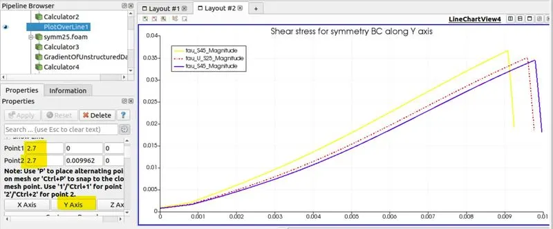
Comparison of Shear stress distribution for Symmetry Boundary conditions at different angles :-

Usage and application of symmetry and wedge boundary condition

Symmetry boundary condition is used for 3D objects under consideration, whereas the wedge boundary condition for axis- symmetric and 2D objects.
symmetry is used in order to reduce the computation time and also the number of cell and complexity.
The conditions for symmetric boundary are no flow across boundary , no scalar flux across boundary.

Conclusion:

The Symmetry BC yields an accurate result for all angles whereas, the Wedge BC yields an accurate result pathway only for the lower order of wedge angles.
It is observed that there isn't any large variation of Kinematic Pressure drop for Symmetry BC, whereas for Wedge BC it shows an oscillating value, and this time the value for pressure for the highest angle is not that accurate when compared to what we inferred in velocity part.

Reference:

Week 12 - Validation studies of Symmetry BC vs Wedge BC in OpenFOAM vs Analytical H.P equation

Ship work like this
in your own course.

Talk to a career counsellor

Ship work like thisin your own course.

Talk to a career counsellor

Ship work like this
in your own course.